

526 | P A R T |
V I More on the Microeconomics Behind Macroeconomics |
|
|
|||||
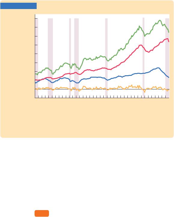
FIGURE 18-1 |
|
|
|
|
|
|
|
|
Billions of |
|
|
|
|
|
|
|
|
2000 dollars 2000 |
|
|
|
|
|
|
|
|
|
1750 |
|
|
|
|
|
|
|
|
1500 |
|
|
|
|
|
|
|
|
1250 |
|
|
|
|
|
|
|
|
1000 |
|
|
Total investment |
|
|
|
|
|
750 |
|
|
Business fixed investment |
|
|
|
|
|
|
|
|
|
|
|
||
|
500 |
|
|
Residential investment |
|
|
|
|
|
|
|
|
|
|
|
||
|
250 |
|
|
Change in inventories |
|
|
|
|
|
|
|
|
|
|
|
||
|
0 |
|
|
|
|
|
|
|
|
250 |
1975 |
1980 |
1985 |
1990 |
1995 |
2000 |
2005 |
|
1970 |
|||||||
|
|
|
|
|
|
|
|
Year |
The Three Components of Investment This figure shows total investment, business fixed investment, residential investment, and inventory investment in the United States from 1970 to 2008. Notice that all types of investment usually fall during recessions, which are indicated here by the shaded areas.
Source: U.S. Department of Commerce and Global Financial Data.
In this chapter we build models of each type of investment to explain these fluctuations. The models will shed light on the following questions:
■Why is investment negatively related to the interest rate?
■What causes the investment function to shift?
■Why does investment rise during booms and fall during recessions?
At the end of the chapter, we return to these questions and summarize the answers that the models offer.
18-1 Business Fixed Investment
The largest piece of investment spending, accounting for about three-quarters of the total, is business fixed investment. The term “business” means that these investment goods are bought by firms for use in future production. The term “fixed” means that this spending is for capital that will stay put for a while, as
C H A P T E R 1 8 Investment | 527
opposed to inventory investment, which will be used or sold within a short time. Business fixed investment includes everything from office furniture to factories, computers to company cars.
The standard model of business fixed investment is called the neoclassical model of investment. The neoclassical model examines the benefits and costs to firms of owning capital goods. The model shows how the level of invest- ment—the addition to the stock of capital—is related to the marginal product of capital, the interest rate, and the tax rules affecting firms.
To develop the model, imagine that there are two kinds of firms in the economy. Production firms produce goods and services using capital that they rent. Rental firms make all the investments in the economy; they buy capital and rent it out to the production firms. Most firms in the real world perform both functions: they produce goods and services, and they invest in capital for future production. We can simplify our analysis and clarify our thinking, however, if we separate these two activities by imagining that they take place in different firms.
The Rental Price of Capital
Let’s first consider the typical production firm. As we discussed in Chapter 3, this firm decides how much capital to rent by comparing the cost and benefit of each unit of capital. The firm rents capital at a rental rate R and sells its output at a price P; the real cost of a unit of capital to the production firm is R/P. The real benefit of a unit of capital is the marginal product of capital MPK—the extra output produced with one more unit of capital. The marginal product of capital declines as the amount of capital rises: the more capital the firm has, the less an additional unit of capital will add to its output. Chapter 3 concluded that, to maximize profit, the firm rents capital until the marginal product of capital falls to equal the real rental price.
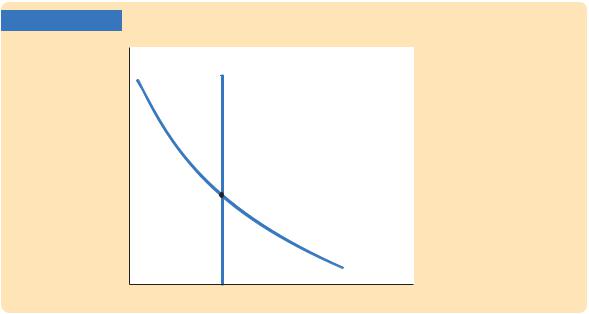
Figure 18-2 shows the equilibrium in the rental market for capital. For the reasons just discussed, the marginal product of capital determines the demand curve. The demand curve slopes downward because the marginal product of capital is low when the level of capital is high. At any point in time, the amount of capital in the economy is fixed, so the supply curve is vertical. The real rental price of capital adjusts to equilibrate supply and demand.
To see what variables influence the equilibrium rental price, let’s consider a particular production function. As we saw in Chapter 3, many economists consider the Cobb–Douglas production function a good approximation of how the actual economy turns capital and labor into goods and services. The Cobb–Douglas production function is
Y = AKaL1−a,
where Y is output, K is capital, L is labor, A is a parameter measuring the level of technology, and a is a parameter between zero and one that measures capital’s share of output. The marginal product of capital for the Cobb–Douglas production function is
MPK = aA(L/K )1−a.
C H A P T E R 1 8 Investment | 529
The cost of owning capital is more complex. For each period of time that it rents out a unit of capital, the rental firm bears three costs:
1.When a rental firm borrows to buy a unit of capital, it must pay interest on
the loan. If PK is the purchase price of a unit of capital and i is the nominal interest rate, then iPK is the interest cost. Notice that this interest cost would be the same even if the rental firm did not have to borrow: if the
rental firm buys a unit of capital using cash on hand, it loses out on the interest it could have earned by depositing this cash in the bank. In either case, the interest cost equals iPK.
2.While the rental firm is renting out the capital, the price of capital can change. If the price of capital falls, the firm loses, because the firm’s asset has
fallen in value. If the price of capital rises, the firm gains, because the firm’s
asset has risen in value. The cost of this loss or gain is −DPK. (The minus sign is here because we are measuring costs, not benefits.)
3.While the capital is rented out, it suffers wear and tear, called depreciation.
If d is the rate of depreciation—the fraction of capital’s value lost per period because of wear and tear—then the dollar cost of depreciation is dPK.
The total cost of renting out a unit of capital for one period is therefore
Cost of Capital = iPK − DPK + dPK
= PK(i − DPK/PK + d).
The cost of capital depends on the price of capital, the interest rate, the rate at which capital prices are changing, and the depreciation rate.
For example, consider the cost of capital to a car-rental company. The company buys cars for $10,000 each and rents them out to other businesses. The company faces an interest rate i of 10 percent per year, so the interest cost iPK is $1,000 per year for each car the company owns. Car prices are rising at 6 percent per year, so, excluding wear and tear, the firm gets a capital gain DPK of $600 per year. Cars depreciate at 20 percent per year, so the loss due to wear and tear dPK is $2,000 per year. Therefore, the company’s cost of capital is
Cost of Capital = $1,000 − $600 + $2,000
= $2,400.
The cost to the car-rental company of keeping a car in its capital stock is $2,400 per year.
To make the expression for the cost of capital simpler and easier to interpret, we assume that the price of capital goods rises with the prices of other goods. In this case, DPK/PK equals the overall rate of inflation p. Because i − p equals the real interest rate r, we can write the cost of capital as
Cost of Capital = PK(r + d).