

CONVERSION FACTORS AND UNIT SYMBOLS
SI UNITS (ADOPTED 1960)
A new system of metric measurement, the International System of Units (abbreviated SI), is being implemented throughout the world. This system is a modernized version of the MKSA (meter, kilogram, second, ampere) system, and its details are published and controlled by an international treaty organization (The International Bureau of Weights and Measures).
SI units are divided into three classes:
Base Units |
|
length |
metery (m) |
massz |
kilogram (kg) |
time |
second (s) |
electric current |
ampere (A) |
thermodynamic temperature§ |
kelvin (K) |
amount of substance |
mole (mol) |
luminous intensity |
candela (cd) |
Supplementary Units |
|
plane angle |
radian (rad) |
solid angle |
steradian (sr) |
Derived Units and Other Acceptable Units
These units are formed by combining base units, supplementary units, and other derived units. Those derived units having special names and symbols are marked with an asterisk (*) in the list below:
Quantity |
Unit |
Symbol |
Acceptable equivalent |
*absorbed dose |
gray |
Gy |
J/kg |
acceleration |
meter per second squared |
m/s2 |
|
*activity (of ionizing radiation source) |
becquerel |
Bq |
1/s |
area |
square kilometer |
km2 |
|
|
square hectometer |
hm2 |
ha (hectare) |
|
square meter |
m2 |
|
yThe spellings ‘‘metre’’ and ‘‘litre’’ are preferred by American Society for Testing and Materials (ASTM); however, ‘‘ er’’ will be used in the Encyclopedia.
z‘‘Weight’’ is the commonly used term for ‘‘mass.’’
§Wide use is made of ‘‘Celsius temperature’’ ðtÞ defined t ¼ T T0 where T is the thermodynamic temperature, expressed in kelvins, and T0 ¼ 273:15 K by definition. A temperature interval may be expressed in degrees Celsius as well as in kelvins.
xxxi
xxxii |
CONVERSION FACTORS AND UNIT SYMBOLS |
|
|
|
|
|
|
|
Quantity |
Unit |
|
Symbol |
Acceptable |
||
|
equivalent |
|
|
|
|
|
|
|
*capacitance |
farad |
|
F |
|
C/V |
|
|
concentration (of amount of substance) |
mole per cubic meter |
mol/m3 |
|
|
||
|
*conductance |
siemens |
|
S |
|
A/V |
|
|
current density |
ampere per square meter |
A/m2 |
|
|
||
|
density, mass density |
kilogram per cubic meter |
kg/m3 |
g/L; mg/cm3 |
|||
|
* |
coulomb meter |
|
|
|
|
|
|
dipole moment (quantity) |
C m |
|
|
|
||
|
electric charge, quantity of electricity |
coulomb |
|
C |
3 |
A s |
|
|
electric charge density |
coulomb per cubic meter |
C/m |
|
|
|
|
|
electric field strength |
volt per meter |
V/m |
|
|
|
|
|
electric flux density |
coulomb per square meter |
C/m2 |
|
|
||
|
*electric potential, potential difference, |
|
|
|
|
|
|
|
electromotive force |
volt |
|
V |
|
W/A |
|
|
*electric resistance |
ohm |
|
V |
|
V/A |
|
|
*energy, work, quantity of heat |
megajoule |
|
MJ |
|
|
|
|
|
kilojoule |
|
kJ |
|
N m |
|
|
|
joule |
|
J |
|
|
|
|
|
electron volty |
y |
eVy |
|
|
|
|
|
|
hy |
|
|
||
|
energy density |
kilowatt hour |
|
kW 3 |
|
|
|
|
joule per cubic meter |
J/m |
|
|
|
||
|
*force |
kilonewton |
|
kN |
|
|
|
|
* |
newton |
|
N |
|
kg m/s2 |
|
|
frequency |
megahertz |
|
MHz |
|
|
|
|
|
hertz |
|
Hz |
|
1/s |
|
|
heat capacity, entropy |
joule per kelvin |
J/K |
K) |
|
|
|
|
heat capacity (specific), specific entropy |
|
|
|
|
|
|
|
heat transfer coefficient |
joule per kilogram kelvin |
J/(kg 2 |
|
|
||
|
watt per square meter |
W/(m K) |
|
|
|||
|
|
kelvin |
|
|
|
|
|
|
*illuminance |
lux |
|
lx |
|
lm/m2 |
|
|
*inductance |
henry |
|
H |
|
Wb/A |
|
|
linear density |
kilogram per meter |
kg/m |
|
|
||
|
luminance |
candela per square meter |
cd/m2 |
cd sr |
|
||
|
*luminous flux |
lumen |
|
lm |
|
|
|
|
magnetic field strength |
ampere per meter |
A/m |
|
|
|
|
|
* |
|
|
|
|
V s |
|
|
*magnetic flux |
weber |
|
Wb |
|
2 |
|
|
magnetic flux density |
tesla |
|
T |
|
Wb/m |
|
|
molar energy |
joule per mole |
J/mol |
|
|
||
|
molar entropy, molar heat capacity |
joule per mole kelvin |
J/(mol K) |
|
|
||
|
moment of force, torque |
newton meter |
N m |
|
|
||
|
momentum |
kilogram meter per second |
kg m/s |
|
|
||
|
permeability |
henry per meter |
H/m |
|
|
||
|
permittivity |
farad per meter |
F/m |
|
|
|
|
|
*power, heat flow rate, radiant flux |
kilowatt |
|
kW |
|
|
|
|
|
watt |
|
W |
|
J/s |
|
|
power density, heat flux density, |
|
|
|
|
|
|
|
irradiance |
watt per square meter |
W/m2 |
|
|
||
|
*pressure, stress |
megapascal |
|
MPa |
|
|
|
|
|
kilopascal |
|
kPa |
|
|
|
|
|
pascal |
|
Pa |
|
N/m2 |
|
|
sound level |
decibel |
|
dB |
|
|
|
|
specific energy |
joule per kilogram |
J/kg |
|
|
||
|
specific volume |
cubic meter per kilogram |
m3/kg |
|
|
||
|
surface tension |
newton per meter |
N/m |
|
|
||
|
thermal conductivity |
watt per meter kelvin |
W/(m K) |
|
|
||
|
velocity |
meter per second |
m/s |
|
|
|
|
|
|
kilometer per hour |
km/h |
|
|
||
|
viscosity, dynamic |
pascal second |
|
Pa s |
|
|
|
|
|
millipascal second |
mPa s |
|
|
||
yThis non-SI unit is recognized as having to be retained because of practical importance or use in specialized fields.
|
CONVERSION FACTORS AND UNIT SYMBOLS |
xxxiii |
||
Quantity |
Unit |
Symbol |
Acceptable equivalent |
|
viscosity, kinematic |
square meter per second |
m2/s |
|
|
|
square millimeter per second |
mm2/s |
|
|
|
cubic meter |
m3 |
|
|
|
cubic decimeter |
dm3 |
L(liter) |
|
|
cubic centimeter |
cm3 |
mL |
|
wave number |
1 per meter |
m 1 |
|
|
|
1 per centimeter |
cm 1 |
|
|
In addition, there are 16 prefixes used to indicate order of magnitude, as follows:
Multiplication factor |
Prefix |
Symbol |
Note |
1018 |
exa |
E |
|
1015 |
peta |
P |
|
1012 |
tera |
T |
|
109 |
giga |
G |
|
108 |
mega |
M |
|
103 |
kilo |
k |
|
102 |
hecto |
ha |
aAlthough hecto, deka, deci, and centi are |
10 |
deka |
daa |
SI prefixes, their use should be avoided |
10 1 |
deci |
da |
except for SI unit-multiples for area and |
10 2 |
centi |
ca |
volume and nontechnical use of |
10 3 |
milli |
m |
centimeter, as for body and clothing |
10 6 |
micro |
m |
measurement. |
10 9 |
nano |
n |
|
10 12 |
pico |
p |
|
10 15 |
femto |
f |
|
10 18 |
atto |
a |
|
For a complete description of SI and its use the reader is referred to ASTM E 380.
CONVERSION FACTORS TO SI UNITS
A representative list of conversion factors from non-SI to SI units is presented herewith. Factors are given to four significant figures. Exact relationships are followed by a dagger (y). A more complete list is given in ASTM E 380-76 and ANSI Z210. 1-1976.
To convert from |
To |
|
|
|
|
Multiply by |
|||
acre |
square meter (m2) |
|
4:047 |
103 |
|||||
angstrom |
meter (m) |
|
2 |
|
|
1:0 |
|
10 10y |
|
|
|
|
|
|
|||||
are |
square meter (m ) |
|
1:0 102y 11 |
||||||
astronomical unit |
meter (m) |
|
|
|
|
1:496 |
105 |
||
atmosphere |
pascal (Pa) |
|
|
|
|
1:013 |
10 |
||
bar |
pascal (Pa) |
3 |
|
|
|
1:0 105y |
|||
barrel (42 U.S. liquid gallons) |
cubic meter (m ) |
|
|
|
0.1590 |
|
|||
|
|
|
|
|
|
1:055 |
3 |
||
Btu (International Table) |
joule (J) |
|
|
|
|
103 |
|||
Btu (mean) |
joule (J) |
|
|
|
|
1:056 |
103 |
||
Bt (thermochemical) |
joule (J) |
3 |
|
|
|
1:054 |
10 |
||
bushel |
cubic meter (m ) |
|
|
|
3:524 |
|
10 2 |
||
|
|
|
|
||||||
calorie (International Table) |
joule (J) |
|
|
|
|
4.187 |
|
|
|
calorie (mean) |
joule (J) |
|
|
|
|
4.190 |
|
|
|
calorie (thermochemical) |
joule (J) |
|
|
|
|
4.184y |
|
||
centimeters of water (39.2 8F) |
pascal (Pa) |
|
|
|
2 |
98.07 |
|
|
|
centipoise |
|
|
|
1:0 |
|
10 3y |
|||
pascal second (Pa s) |
|
|
|||||||
centistokes |
square millimeter per second (mm /s) |
1.0y |
|
|
|||||
xxxiv CONVERSION FACTORS AND UNIT SYMBOLS
To convert from |
To |
|
|
|
|
Multiply by |
||||||
cfm (cubic foot per minute) |
|
3 |
|
|
|
4:72 |
|
10 4 |
||||
cubic meter per second (m3/s) |
|
|
|
|||||||||
cubic inch |
cubic meter (m3) |
|
|
|
1:639 |
10 4 |
||||||
cubic foot |
cubic meter (m3) |
|
|
|
2:832 |
10 2 |
||||||
cubic yard |
cubic meter (m ) |
|
|
|
0.7646 |
|
|
|
||||
curie |
becquerel (Bq) |
|
|
|
|
3:70 1010y |
||||||
debye |
|
|
|
|
3:336 |
|
10 30 |
|||||
coulomb-meter (C m) |
|
|
||||||||||
degree (angle) |
radian (rad) |
|
|
|
|
1:745 |
10 2 |
|||||
|
|
|
|
|
|
|||||||
denier (international) |
kilogram per meter (kg/m) |
|
1:111 |
10 7 |
||||||||
|
tex |
|
|
|
|
0.1111 |
|
|
|
|||
dram (apothecaries’) |
kilogram (kg) |
|
|
|
|
3:888 |
|
10 3 |
||||
|
|
|
|
|
|
|||||||
dram (avoirdupois) |
kilogram (kg) |
3 |
|
|
|
1:772 |
10 3 |
|||||
dram (U.S. fluid) |
cubic meter (m ) |
|
|
|
3:697 |
10 6 |
||||||
dyne |
newton(N) |
|
|
|
|
1:0 10 6y |
||||||
dyne/cm |
newton per meter (N/m) |
|
1:00 10 3y |
|||||||||
electron volt |
joule (J) |
|
|
|
|
1:602 |
10 19 |
|||||
erg |
joule (J) |
|
|
|
|
1:0 10 7y |
||||||
fathom |
meter (m) |
|
|
|
|
1.829 |
|
|
|
|
||
fluid ounce (U.S.) |
cubic meter (m3) |
|
|
|
2:957 |
10 5 |
||||||
foot |
meter (m) |
|
|
|
|
0.3048y |
|
|
||||
foot-pound force |
joule (J) |
|
|
|
|
1.356 |
|
|
|
|
||
foot-pound force |
newton meter (N m) |
|
1.356 |
|
|
|
|
|||||
foot-pound force per second |
watt(W) |
|
|
|
|
1.356 |
|
|
|
|
||
footcandle |
lux (lx) |
|
|
|
|
10.76 |
|
|
|
|
||
furlong |
meter (m) |
3 |
|
2 |
|
2:012 |
102 |
|||||
gal |
|
|
|
|
1:0 |
|
10 2y |
|||||
meter per second squared (m/s ) |
|
|
||||||||||
gallon (U.S. dry) |
cubic meter (m3) |
|
|
|
4:405 |
10 3 |
||||||
gallon (U.S. liquid) |
cubic meter (m ) |
|
|
|
3:785 |
10 3 |
||||||
gilbert |
ampere (A) |
|
|
|
|
0.7958 |
|
|
|
|||
gill (U.S.) |
cubic meter (m3) |
|
|
|
1:183 |
|
10 4 |
|||||
grad |
radian |
|
|
|
|
1:571 |
|
10 2 |
||||
|
|
|
|
|
||||||||
grain |
kilogram (kg) |
|
|
|
|
6:480 |
10 5 |
|||||
|
2 |
|
|
|
||||||||
gram force per denier |
|
|
|
|
8:826 |
10 2 |
||||||
newton per tex (N/tex) |
|
|
|
|||||||||
hectare |
square meter (m ) |
|
1:0 104y |
2 |
||||||||
horsepower (550 ft lbf/s) |
watt(W) |
|
|
|
|
7:457 |
103 |
|||||
horsepower (boiler) |
watt(W) |
|
|
|
|
9:810 |
10 |
|
||||
horsepower (electric) |
watt(W) |
|
|
|
|
7:46 102y |
||||||
hundredweight (long) |
kilogram (kg) |
|
|
|
|
50.80 |
|
|
|
|
||
hundredweight (short) |
kilogram (kg) |
|
|
|
|
45.36 |
|
|
|
3 |
||
inch |
meter (m) |
|
|
|
|
2:54 |
|
|
|
|||
|
|
|
|
|
|
10 2y |
||||||
inch of mercury (32 8F) |
pascal (Pa) |
|
|
|
|
3:386 |
102 |
|||||
inch of water (39.2 8F) |
pascal (Pa) |
|
|
|
|
2:491 |
10 |
|
||||
kilogram force |
newton (N) |
|
|
|
|
9.807 |
|
|
|
|
||
kilopond |
newton (N) |
|
|
|
|
9.807 |
|
|
|
|
||
kilopond-meter |
newton-meter (N m) |
|
9.807 |
|
|
|
|
|||||
kilopond-meter per second |
watt (W) |
|
|
|
|
9.807 |
|
|
|
|
||
kilopond-meter per min |
watt(W) |
|
|
|
|
0.1635 |
|
|
|
|||
kilowatt hour |
megajoule (MJ) |
|
|
|
3.6y |
|
|
|
|
|
||
kip |
newton (N) |
|
|
|
|
4:448 |
102 |
|||||
knot international |
meter per second (m/s) |
|
0.5144 |
|
|
|
||||||
lambert |
candela per square meter (cd/m |
2 |
3:183 |
|
3 |
|||||||
) |
102 |
|||||||||||
league (British nautical) |
meter (m) |
|
|
|
|
5:559 |
103 |
|||||
league (statute) |
meter (m) |
|
|
|
|
4:828 |
1015 |
|||||
light year |
meter (m) |
3 |
|
|
|
9:461 |
10 |
|
||||
liter (for fluids only) |
cubic meter (m ) |
|
|
|
1:0 |
|
10 3y |
|||||
maxwell |
weber (Wb) |
|
|
|
|
1:0 |
|
10 8y |
||||
|
|
|
|
|
|
|||||||
micron |
meter (m) |
|
|
|
|
1:0 10 6y |
||||||
mil |
meter (m) |
|
|
|
|
2:54 10 5y |
||||||
mile (U.S. nautical) |
meter (m) |
|
|
|
|
1:852 |
|
|
3 |
|||
|
|
|
|
|
|
103y |
||||||
mile (statute) |
meter (m) |
|
|
|
|
1:609 |
10 |
|
||||
mile per hour |
meter per second (m/s) |
|
0.4470 |
|
|
|
||||||
|
|
|
|
CONVERSION FACTORS AND UNIT SYMBOLS |
xxxv |
||||
To convert from |
To |
|
|
|
Multiply by |
||||
millibar |
pascal (Pa) |
|
|
|
1:0 102 |
|
|||
millimeter of mercury (0 8C) |
pascal (Pa) |
|
|
|
1:333 |
102y |
|||
millimeter of water (39.2 8F) |
pascal (Pa) |
|
|
|
9.807 |
|
|
|
|
minute (angular) |
radian |
|
|
|
2:909 |
10 4 |
|||
|
|
|
|
||||||
myriagram |
kilogram (kg) |
|
|
|
10 |
|
|
|
|
myriameter |
kilometer (km) |
|
|
|
10 |
|
|
|
|
oersted |
ampere per meter (A/m) |
79.58 |
|
|
|
||||
ounce (avoirdupois) |
kilogram (kg) |
|
|
|
2:835 |
10 2 |
|||
|
|
|
|
||||||
ounce (troy) |
kilogram (kg) |
3 |
|
|
3:110 |
10 2 |
|||
ounce (U.S. fluid) |
cubic meter (m ) |
|
|
2:957 |
10 5 |
||||
ounce-force |
newton (N) |
|
|
|
0.2780 |
|
|
||
peck (U.S.) |
cubic meter (m3) |
|
|
8:810 |
|
10 3 |
|||
|
|
|
|||||||
pennyweight |
kilogram (kg) |
|
|
|
1:555 |
|
10 3 |
||
pint (U.S. dry) |
cubic meter (m3) |
|
|
5:506 |
10 4 |
||||
pint (U.S. liquid) |
cubic meter (m3) |
|
|
4:732 |
|
10 4 |
|||
|
|
|
|||||||
poise (absolute viscosity) |
pascal second (Pa s) |
0.10y |
|
|
|
||||
pound (avoirdupois) |
kilogram (kg) |
|
|
|
0.4536 |
|
|
||
pound (troy) |
kilogram (kg) |
|
|
|
0.3732 |
|
|
||
poundal |
newton (N) |
|
|
|
0.1383 |
|
|
||
pound-force |
newton (N) |
|
|
|
4.448 |
|
|
|
|
pound per square inch (psi) |
pascal (Pa) |
3 |
|
|
6:895 |
103 |
|||
quart (U.S. dry) |
cubic meter (m3) |
|
|
1:101 |
10 3 |
||||
quart (U.S. liquid) |
cubic meter (m ) |
|
|
9:464 |
10 4 |
||||
quintal |
kilogram (kg) |
|
|
|
1:0 |
|
102y |
|
|
|
|
|
|
|
|||||
rad |
gray (Gy) |
|
|
|
1:0 10 2y |
||||
rod |
meter (m) |
|
|
|
5.029 |
|
|
|
|
roentgen |
coulomb per kilogram (C/kg) |
2:58 10 4 |
|||||||
second (angle) |
radian (rad) |
|
2 |
|
4:848 |
|
|
6 |
|
|
|
|
|
10 6 |
|||||
section |
square meter (m ) |
2:590 |
10 |
|
|||||
slug |
kilogram (kg) |
|
|
|
14.59 |
|
|
|
|
spherical candle power |
lumen (lm) |
|
|
|
12.57 |
|
|
|
|
square inch |
square meter (m2) |
6:452 10 4 |
|||||||
square foot |
|
|
2 |
|
9:290 |
|
|
6 |
|
square meter (m2) |
|
10 2 |
|||||||
square mile |
square meter (m2) |
2:590 |
10 |
|
|||||
square yard |
square meter (m ) |
0.8361 |
|
|
|||||
store |
cubic meter (m3) |
|
|
1:0y |
|
|
|
||
stokes (kinematic viscosity) |
square meter per second (m2/s) |
1:0 |
|
10 4y |
|||||
tex |
kilogram per meter (kg/m) |
1:0 |
|
|
|
3 |
|||
|
10 6y |
||||||||
ton (long, 2240 pounds) |
kilogram (kg) |
|
|
|
1:016 |
10 |
|
||
ton (metric) |
kilogram (kg) |
|
|
|
1:0 103y |
2 |
|||
ton (short, 2000 pounds) |
kilogram (kg) |
|
|
|
9:072 |
102 |
|||
torr |
pascal (Pa) |
|
|
|
1:333 |
10 |
|
||
unit pole |
weber (Wb) |
|
|
|
1:257 |
10 7 |
|||
yard |
meter (m) |
|
|
|
0.9144y |
|
|
||

E
ECG. See ELECTROCARDIOGRAPHY, COMPUTERS IN.
ECHOCARDIOGRAPHY AND DOPPLER ECHOCARDIOGRAPHY
PETER S. RAHKO
University of Wisconsin Medical
School
Madison, Wisconsin
INTRODUCTION
Echocardiography is a diagnostic technique that utilizes ultrasound (high frequency sound waves above the audible limit of 20 kHz) to produce an image of the beating heart in real time. A piezoelectric transducer element is used to emit short bursts of high frequency, low intensity sound through the chest wall to the heart and then detect the reflections of this sound as it returns from the heart. Since movement patterns and shape changes of several regions of the heart correlate with cardiac function and since changes in these patterns consistently appear in several types of cardiac disease, echocardiography has become a frequently used method for evaluation of the heart. Echocardiography has several advantages over other diagnostic tests of cardiac function:
1. It is flexible and can be used with transducers placed on the chest wall, inside oral cavities such as the esophagus or stomach, or inside the heart and great vessels.
2. It is painless.
3. It is a safe procedure that has no known harmful biologic effects.
4. It is easily transported almost anywhere including the bedside, operating room, cath lab, or emergency department.
5. It may be repeated as frequently as necessary allowing serial evaluation of a given disease process.
6. It produces an image instantaneously, which allows rapid diagnosis in emergent situations.
The first echocardiogram was performed by Edler and Hertz in 1953 (1) using a device that displayed reflected ultrasound on a cathode ray tube. Since that time multiple interrogation and display formats have been devised to display reflected ultrasound. The common display formats are
M-mode: A narrow beam of reflected sound is displayed on a scrolling strip chart plotting depth versus time. Only a small portion of the heart along one interrogation line (‘‘ice pick’’ view) is shown at any one time.
Two-Dimensional Sector Scan (2D): A sector scan is generated by sequential firing of a phased array transducer along different lines of sight that are swept through a 2D plane. The image (a narrow plane in cross-section) is typically updated at a rate of 15–200 Hz and shown on a video monitor, which allows real time display of cardiac motion.
Three-Dimensional Imaging (3D): Image data from multiple 2D sector scans are acquired sequentially or in real time and displayed in a spatial format in three dimensions. If continuous data is displayed, time becomes the fourth dimension. The display can be shown as a loop that continuously repeats or on some systems in real time. Software allows rotation and ‘‘slicing’’ of the display.
Doppler: The Doppler effect is used to detect the rate and direction of blood flowing in the chambers of the heart and great vessels. Blood generally moves at a higher velocity than the walls of cardiac structures allowing motion of these structures to be filtered out. Blood flow is displayed in four formats:
Continuous Wave Doppler (CW): A signal of continuous frequency is directed into the heart while a receiver (or array of receivers) continuously processes the reflected signal. The difference between the two signals is processed and displayed showing direction and velocity of blood flow. All blood velocities in the line of sight of the Doppler beam are displayed.
Pulsed Wave Doppler (PW): Many bursts of sound are transmitted into the heart and reflected signals from a user defined depth are acquired and stored for each burst. Using these reflected signals an estimate is made of the velocities of blood or tissue encountered by the burst of sound at the selected depth. The velocity estimates are displayed similar to CW Doppler. The user defined position in the heart that the signal is obtained from stipulate the time of the acquisition of the reflected signal relative to transmission and length of the burst, respectively. The difference between transmitted and reflected signal frequencies is calculated, converted to velocity, and displayed. By varying the time between transmission and reception of the signal, selected velocities in small parts of the heart are sampled for blood flow.
Duplex Scanning: The 2D echo is used to orient the interrogator to the location of either the CW or PW signal allowing rapid correlation of blood flow data with cardiac anatomy. This is done by simultaneous display of the Doppler positional range gate superimposed on the 2D image.
Color Doppler: Using a complex array of bursts of frequency (pulsed packets) and multiple ultrasound acquisitions down the same beam line, motion of blood flow is estimated from a cross-correlation among the various acquired reflected waves. The
1
2 ECHOCARDIOGRAPHY AND DOPPLER ECHOCARDIOGRAPHY
data is combined as an overlay onto the 2D sector scan for anatomical orientation. Blood flow direction, and an estimate of flow velocity are displayed simultaneously with 2D echocardiographic data for each point in the sector.
CLINICAL FORMATS OF ULTRASOUND
Current generation ultrasound systems allow display of all of the imaging formats discussed except 3D/4D imaging that is still limited in availability to some high end systems.
Specialized transducers that emit and receive the ultrasound have been designed for various clinical indications. Four common types of transducers are used (Fig. 1):
Transthoracic: By far the most common, this transducer is placed on the surface of the chest and moved to different locations to image different parts of the heart or great vessels. All display formats are possible (Fig. 2).
Transesophageal: The transducer is designed to be inserted through the patient’s mouth into the esophagus and stomach. The ultrasound signal is directed at the heart from that location for specialized exams. All display formats are possible.
Intracardiac: A small transducer is mounted on a catheter, inserted into a large vein and moved into the heart. Imaging from within the heart is performed to monitor specialized interventional therapy. Most display formats are available.
Intravascular: Miniature sized transducers are mounted on small catheters and moved through arteries to examine arterial pathology and the results of selected interventions. Limited 2D display formats are available some being radial rather than sector based. The transducers run at very high frequencies (20–30 MHz).
Ultrasound systems vary considerably in size and sophistication (Fig. 3). Full size systems, typically found in hospitals display all imaging formats, accept all types of
Figure 1. Comparative view of commonly used ultrasound transducers: (a) intracardiac, (b) transesophageal, (c) transthoracic, and
(d) Pedof (special Doppler) transducer. A pencil is shown for size reference.
Suprasternal
 Sternal notch
|
|
Parasternal |
Ao |
|
Assume left side |
|
unless otherwise stated |
|
|
PA |
|
|
|
|
|
|
LA |
RA
LV
LAXX
RV
SAXX
|
|
Apical |
|
|
|
Assume left side |
|
Subcostal |
|||
unless otherwise stated |
|||
|
|
||
(b)
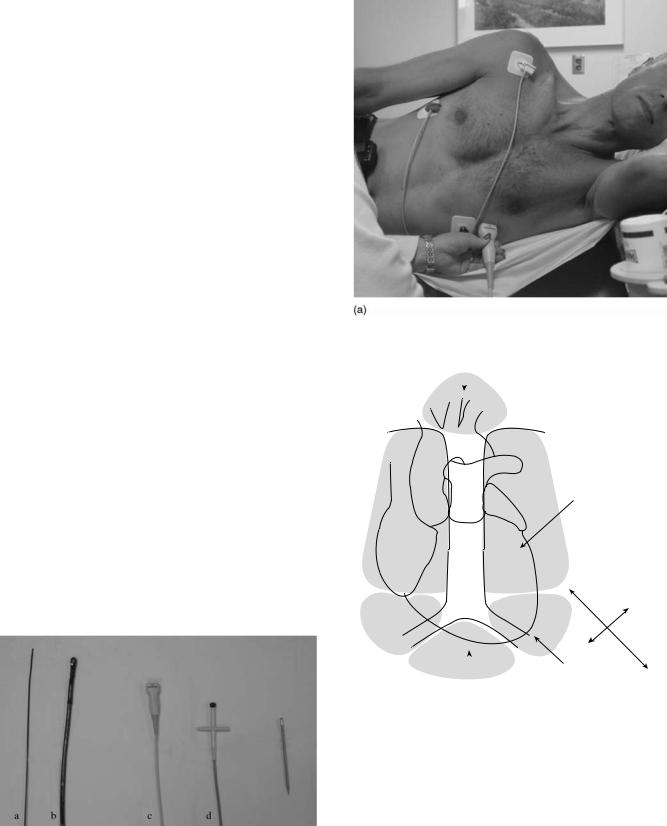
Figure 2. (a) Phased array transducer used for transthoracic imaging. The patient is shown, on left side, on exam table, typical for a transthoracic study. The transducer is in the apical position.
(b) Diagram of the chest showing how the heart and great vessels are positioned in the chest and the locations where transthoracic transducers are placed on the chest wall. The four common positions for transducer placement are shown. The long axis (LAXX) and short axis (SAXX) orientations of the heart are shown for reference. These orientations form a reference for all of the views obtained in a study. Abbreviations are as follows: aorta (Ao), left atrium (LA), left ventricle (LV), pulmonary artery (PA), right atrium (RA), and right ventricle (RV).
ECHOCARDIOGRAPHY AND DOPPLER ECHOCARDIOGRAPHY |
3 |
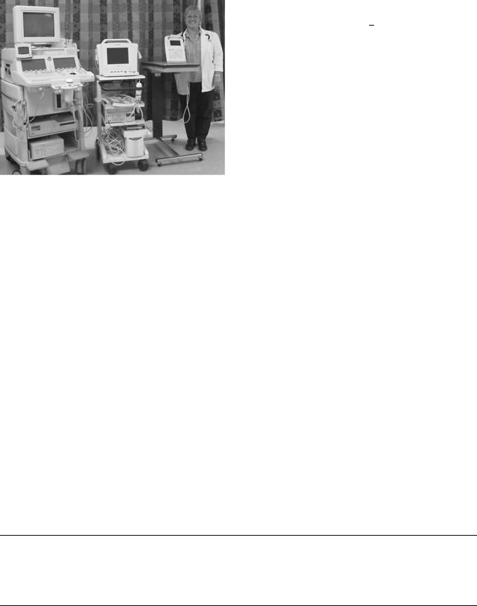
Figure 3. Picture showing various types of ultrasound systems. At left a large ‘‘full-size’’ system is shown that can perform all types of imaging. At center is a miniaturized system that has most of the features of the full service system, but limited display, analysis and recording formats are available. The smallest ‘‘hand-held’’ system shown at right has basic features and is battery operated. It is designed for rapid screening exams integrated into a clinical assessment at the bedside, clinic, or emergency room.
transthoracic and transesophageal transducers, allow considerable on line image processing and support considerable analytic capacity to quantify the image.
Small imaging systems accept many but not all transducers and produce virtually all display formats, but lack the sophisticated array of image processing and analysis capacity found on the full systems. These devices may be used in ambulatory offices or other specialized circumstances requiring more basic image data. A full clinical study is possible.
Portable hand-held battery operated devices are used in limited circumstances, sometimes for screening exams or limited studies. Typically transducers are limited, image processing is rudimentary and analysis capacity very limited.
PRINCIPLES OF ULTRASOUND
Prior to discussing the mechanism of image production some common terms that govern the behavior of ultrasound in soft tissue should be defined. Since ultrasound is
propagated in waves, its behavior in a medium is defined by
l ¼ fc
where f is the wave frequency, l is the wavelength, and c is the acoustic velocity of ultrasound in the medium. The acoustic velocity for most soft tissues is similar and remains constant for a given tissue no matter what the frequency or wavelength (Table 1). Thus in any tissue frequency and wavelength are inversely related. As frequency increases, wavelength decreases. As wavelength decreases, the minimum distance between two structures, that allows them to be characterized as two separate structures, also decreases. This is called the spatial resolution of the instrument. One might conclude that very high frequency should always be used to maximize resolution. Unfortunately, as frequency increases, penetration of the ultrasound signal into soft tissue decreases. This serves to limit the frequency and, thus, the resolving power of an ultrasonic system for any given application.
Sound waves are emitted in short bursts from the transducer. As frequency rises, it takes less time to emit the same number of waves per burst. Thus, more bursts of sound can be emitted per unit of time, increasing the spatial resolution of the instrument (Fig. 4). The optimal image is generated by using a frequency that gives the highest possible resolution and an adequate amount of penetration. For transthoracic transducers expected to penetrate up to 24 cm into the chest, typical frequencies used are from 1.6 to 7.0 MHz. Most transducers are broadband in that they generate sound within an adjustable range of frequency rather than at a single frequency. Certain specialized transducers such as the intravascular transducer may only need to penetrate 4 cm. They may have a frequency of 30 MHz to maximize resolution of small structures.
The term ultrasonic attenuation formally defines the more qualitative concept of tissue penetration. It is a complex parameter that is different for every tissue type and is defined as the rate of decrease in wave amplitude per distance penetrated at a given frequency. The two important properties that define ultrasonic attenuation are reflection and absorption of sound waves (2). Note in Table 1 that ultrasound easily passes through blood and soft tissue, but poorly penetrates bone or air-filled lungs.
Acoustic impedance (z) is the product of acoustic velocity (c) and tissue density (r); thus this property is tissue specific but frequency independent. This property is important because it determines how much ultrasound is
Table 1. Ultrasonic Properties of Some Selected Tissuesa
Tissue |
Velocity of Propagation, 103 m s 1 |
Density, g mL 1 |
Acoustic Impedance, l06 raylb |
Attenuation at 2.25 MHz, dB cm 1 |
Blood |
1.56 |
1.06 |
1.62 |
0.57 |
Myocardium |
1.54 |
1.07 |
1.67 |
3 |
Fat |
1.48 |
0.92 |
1.35 |
1.7 |
Bone |
3–4 |
1.4–1.8 |
4–6 |
37 |
Lung (inflated) |
0.7 |
0.4 |
0.26–0.46 |
62 |
aAdapted from Wilson D. A., Basic principles of ultrasound. In: Kraus R., editor. The Practice of Echocardiography, New York: John Wiley & Sons; 1985, p 15.
This material is used by permission of John Wiley & Sons, Inc. b1 rayl ¼ 1 kg m 2 s 1.
4 ECHOCARDIOGRAPHY AND DOPPLER ECHOCARDIOGRAPHY
l
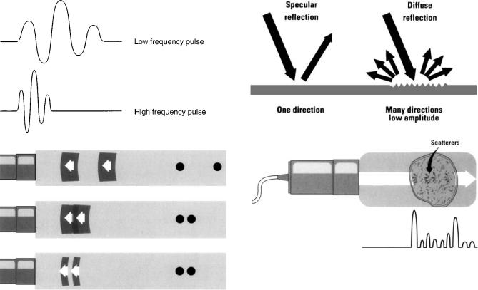
Figure 4. Upper panel Two depictions of an emitted pulse of ultrasound. Time moves horizontally and amplitude moves vertically. Note the high frequency pulse of three waves takes less time. Lower panel Effect of pulse duration on resolution. One echo pulse is delivered toward two reflectors and reflections are shown. In the top panel, the reflectors are well separated from each other and distinguished as two separate structures. In the middle panel, pulse frequency and duration are unchanged, but the reflectors are close together. The two returning reflections overlap, the instrument will register the two reflectors as one structure. In the lower panel the pulse frequency is increased, thus pulse duration is shortened. The two objects are again separately resolved. (Reprinted from Zagzebski JA Essentials of Ultrasound Physics. St. Louis: Mosby-Year Book; copyright # 1996, p 28, with permission from Elsevier.)
reflected at an interface between two different types of tissue (Table 1). When a short burst of ultrasound is directed at the heart, portions of this energy are reflected back to the receiver. It is these reflected waves that produce the image of the heart. A very dense structure such as calcified tissue has high impedance and is a strong reflector.
There are two types of reflected waves: specular reflections and diffuse reflections (Fig. 5). Specular reflections occur at the interface between two types of tissue. The greater the difference in acoustic impedance between two tissues, the greater the amount of specular reflection and the lower the amount of energy that penetrates beyond the interface. The interface between heart muscle and blood produces a specular echo, as does the interface between a heart valve and blood. Specular echoes are the primary
Figure 5. Upper panel Comparison between specular and diffuse reflectors. Note the diffuse reflector is less angle dependent than the specular reflector. Lower panel Example of combined reflections (shown at bottom of figure) returning from a structure, typical of reflections coming back from heart muscle. The large amplitude specular echo corresponds to the border of the structure. The interior of the structure produces low amplitude scattered reflections. (Reprinted from Zagzebski JA, Essentials of Ultrasound Physics. St. Louis, Mosby-Year Book; copyright # 1996 p 12 with permission from Elsevier.)
echoes that are imaged by M-mode, 2D echo, and 3D echo and thus primarily form an outline of the heart. Diffuse reflected echoes are much weaker in energy. They are produced by small irregular more weakly reflective objects such as the myocardium itself. Scattered echoes ‘‘fill in the details’’ between the specular echoes. With modern equipment scattered echoes are processed and analyzed providing much more detail to tissue being examined.
Doppler echocardiography uses scattered echoes from red blood cells for detecting blood flow. Blood cells are Rayleigh scatterers since the diameter of the blood cells are much smaller than the typical wavelength of sound used to interrogate tissue. Since these reflected signals are even fainter than myocardial echoes, Doppler must operate at a higher energy level than M-mode or 2D imaging.
Harmonic imaging is a recent addition to image display made possible by advances in transducer design and signal processing. It was first developed to improve the display of contrast agents injected intravenously as they passed through the heart. These agents, gas filled microbubbles 2–5 mm in diameter, are highly reflective Rayleigh scatterers. At certain frequencies within the broadband transducer range the contrast bubbles resonate, producing a relatively strong signal at multiples of the fundamental interrogation frequency called harmonics. By using a high
pass filter (a system that blanks out all frequency below a certain level), to eliminate the fundamental frequency reflectors, selective reflections from the second harmonic are displayed. In second harmonic mode, reflections from the resonating bubbles are a much stronger than reflections from soft tissue and thus bubbles are preferentially displayed. This allows selective analysis of the contrast agent as it passes through the heart muscle or in the LV cavity (3).
Harmonic imaging has recently been applied to conventional 2D images without contrast. As the ultrasound wave passes through tissue, the waveform is modified by nonlinear propagation through tissue causing a shape change in the ultrasound beam. This progressively increases as the beam travels deeper into the heart. Electronic canceling of much of the image by filtering out the fundamental frequency allows selective display of the harmonic image, improving overall image quality by elimination of some artifacts. The spatial resolution of the signal is also improved since the reflected signal analyzed and displayed is double that of the frequency produced by the transducer (4).
ECHOCARDIOGRAPHIC INSTRUMENTATION
The transducer is a piezoelectric (pressure electric) device. When subjected to an alternating electrical current, the ceramic crystal (usually barium titanate, lead zirconate titanate, or a composite ceramic) expands and contracts producing compressions and rarefactions in its environment, which become waves. Various transducers produce ultrasonic waves within a frequency range of 1.0–40 MHz. The waves are emitted as brief pulses lasting 1 ms out of every 100–200 ms. During the remaining 99–199 ms of each interval the transducer functions as a receiver that detects specular and diffuse reflections as they return from the heart. The same crystal, when excited by a reflected sound wave, produces an electrical signal and sends it back to the echocardiograph for analysis and display. Since one heartbeat lasts somewhere from 0.3 to 1.2 s, the echocardiographic device sends out a minimum of several hundred impulses per beat allowing precise tracking of cardiac motion throughout the beat.
After the specular and diffuse echoes are received they must be displayed in a usable format. The original ultrasound devices used an A-mode format (Fig. 6) that displayed depth on the y axis and amplitude of the signal on the x-axis. The specular echoes from boundaries between cardiac chambers register as the strongest echoes. No more than 1D spatial information is obtained from this format.
In a second format, B-mode, the amplitudes of the returning echoes are displayed as dots of varying intensity on a video monitor in what has come to be called a gray scale (Fig. 6). If the background is black (zero intensity), then progressively stronger echoes are displayed as progressively brighter shades of gray with white representing the highest intensity. Most echocardiographic equipment today uses between 64 and 512 shades of gray in its output display. The B-mode format, by itself, is not adequate for cardiac imaging and must be modified to image a continuously moving structure.
ECHOCARDIOGRAPHY AND DOPPLER ECHOCARDIOGRAPHY |
5 |
Figure 6. Composite drawing showing the three different modes of display for a one-dimensional (1D) ultrasound signal. In the right half of the figure is a schematic drawing of a cross-section through the heart. The transducer (T) sits on the chest wall (CW) and directs a thin beam of ultrasonic pulses into the heart. This beam traverses the anterior wall (aHW) of the right ventricle (RV), the interventricular septum (IVS), the anterior (aML), and posterior (pML) leaflets of the mitral valve, and the posterior wall of the left ventricle (LVPW). Each dot along the path of the beam represents production of a specular echo. These are displayed in the corresponding A-mode format, where vertical direction is depth and horizontal direction is amplitude of the reflected echo and B- mode format where again vertical direction is depth but amplitude is intensity of the dot. If time is added to the B-mode format, an M-mode echo is produced, which is shown in the left panel. This allows simultaneous presentation of motion of the cardiac structures in the path of the echo beam throughout the entire cardiac cycle; measurement of vertical depth, thickness of various structures, and timing of events within the cardiac cycle. If the transducer is angled in a different direction, a distinctly different configuration of echoes will be obtained. In the figure, the M-mode displayed is at the same beam location as noted in the right-side panel. Typical movement of the AML and PML is shown. ECG ¼ electrocardiogram signal. (From Pierand L., Meltzer RS., Roelandt J, Examination techniques in M-mode and twodimensional echocardiography. In: Kraus R editor, The Practice of Echocardiography, New York: John Wiley & Sons; copyright # 1985, p 69. This material is used by permission of John Wiley & Sons, Inc.)
To image the heart, the M-mode format (M for motion) was devised (Fig. 6). With this technique, the transducer is pointed into the chest at the heart and returning echoes are displayed in B-mode. A strip chart recorder (or scrolling video display) constantly records the B-mode signal with depth of penetration on the y-axis and time the parameter displayed on the x-axis. By adding an electrocardiographic signal to monitor cardiac electrical activity and to mark the beginning of each cardiac cycle, the size, thickness, and movement of various cardiac structures throughout a cardiac cycle are displayed with high resolution. By variation of transducer position, the ultrasound beam is directed toward several cardiac structures (Fig. 7).
The M-mode echo was the first practical ultrasound device for cardiac imaging and has produced a considerable amount of important data. Its major limitation is its limited field of view. Few spatial relationships between cardiac structures can be displayed that severely limits diagnostic capability. The angle of interrogation of the heart is also
6 ECHOCARDIOGRAPHY AND DOPPLER ECHOCARDIOGRAPHY
Figure 7. Upper panel Schematic diagram of the heart as in Fig. 6. The principal M-mode views are labeled 1–4. The corresponding M-mode image from these four views is shown in lower panel Abbreviations as in Fig. 6a Additional abbreviations: AV ¼ Aortic valve, AAOW ¼ anterior aortic wall, LA ¼ left atrial posterior wall, LVOT ¼ left ventricular outflow tract, RVOT ¼ right ventricular outflow tract. (From Pierand L, Meltzer RS, Roelandt J, Examination techniques in M-mode and 2D echocardiography. In: Kraus R editor, The Practice of Echocardiography, New York, John Wiley & Sons; copyright # 1985, p 71. This material is used with permission of John Wiley & Sons, Inc.)
difficult to control. This can distort the image and render size and dimension measurements unreliable.
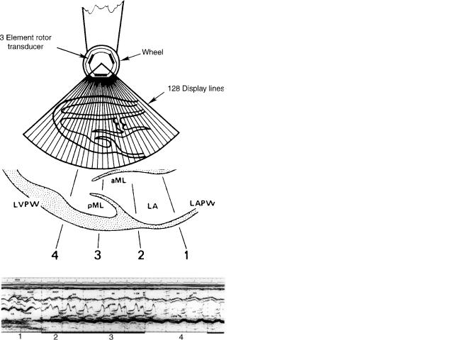
Since the speed of sound is rapid enough to allow up to 5000 short pulses of ultrasound to be emitted and received each second at depths typical for cardiac imaging, it was recognized that multiple B-mode scans in several directions could be processed rapidly enough to display a ‘‘real-time’’ image. Sector scanning in two dimensions was originally performed by mechanically moving a single element piezoelectric crystal through a plane. Typically, 128 B-mode scan lines were swept through a 60–908 arc 30 times s 1 to form a video composite B-mode sector (Fig. 8). These mechanical devices have been replaced by transducer arrays that place a group of closely spaced piezoelectric elements, each with its own electrical connection to the ultrasound system, into a transducer. The type of array used depends on the structure
Figure 8. Diagram of a 2D echo mechanical transducer with three crystals. As each segment sweeps through the 908 arc, an element fires a total of 128 times. The composite of the 128 B-mode lines form a 2D echo frame. Typically there are 30 frames/s of video information, a rate rapid enough to show contractile motion of the heart smoothly. (From Graham PL, Instrumentation. In: Krause R. editor. The Practice of Echocardiography, New York: John Wiley & Sons; copyright # 1985, p 41. This material is used by permission of John Wiley & Sons, Inc.)
being imaged. For cardiac ultrasound, a phased array configuration is used, typically consisting of 128–1024 individual elements. In a phased array transducer, a portion of the elements are fired to produce each sector scan line. The sound beams are electronically steered through the sector by changing the time delay sequence of the array elements (Fig. 9). In a similar fashion, all elements are electronically sequenced to receive reflected sound from selected parts of the sector being scanned (5).
Use of a phased array device allows many other modifications of the sound wave in addition to steering. Further sophisticated electronic manipulations of the time of sound transmission and delays in reception allow selective focusing of the beam to concentrate transmit energy that enhance image quality of selected structures displaced in the sector. Recent design advances have markedly increased the sector frame rate (number of displayed sectors/second) to levels beyond 220 Hz, markedly increasing the time resolution of the imaging system. While the human visual processing system cannot resolve time at such a rapid rate, high frame rates allow for sophisticated quantitation based on the 2D image, such as high-resolu- tion graphs of time based indexes.
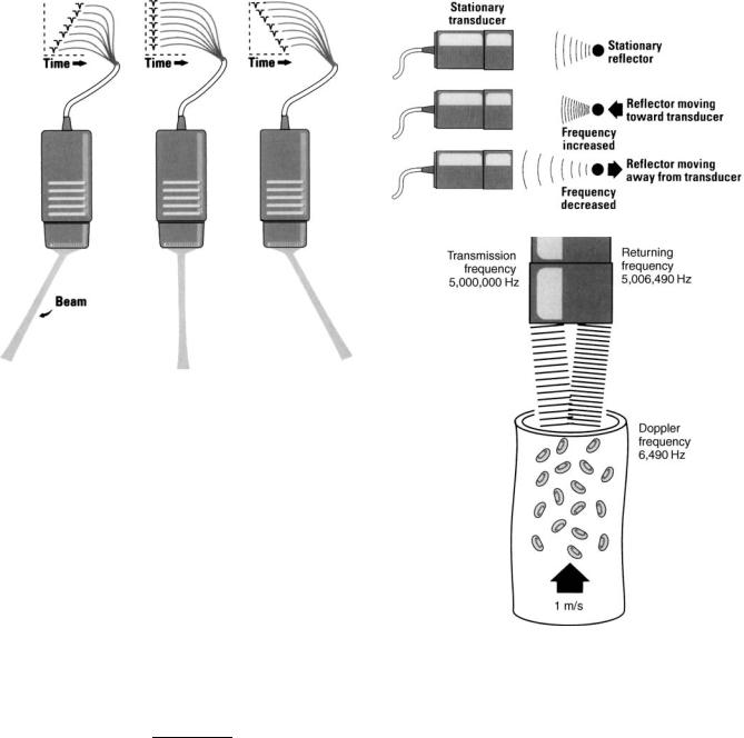
DOPPLER ECHOCARDIOGRAPHY
Application of the Doppler effect allows analysis of blood flow within the heart and great vessels. The Doppler effect, named for its discoverer Christian Doppler, describes the change in frequency and wavelength that occurs with relative motion between the source of the waves and the receiver. If a source of sound remains stationary with respect to its listener, then the frequency and wavelength of the sound will also remain constant. However, if the
ECHOCARDIOGRAPHY AND DOPPLER ECHOCARDIOGRAPHY |
7 |
Figure 9. Diagram of a phased array transducer. Beam direction is varied by changing the delay sequence among the transmitted pulses produced by each individual element. (From Zagzebski JA. Essentials of Ultrasound Physics. St. Louis: Mosby-Year Book Inc.; copyright # 1996, with permission from Elsevier.)
sound source is moving away from the listener wavelength increases and frequency decreases. The opposite will occur if the sound source is moving toward the listener (Fig. 10).
The Doppler principle is applied to cardiac ultrasound in the following way: A beam of continuous wave ultrasound is transmitted into the heart and reflected off red blood cells as they travel through the heart. The reflected impulses are then detected by a receiver. If the red blood cells are moving toward the receiver, the frequency of the reflected echoes will be higher than the frequency of the transmitted echoes and vice versa (Fig. 10).
The difference between the frequency of the transmitted and received echoes (usually called the Doppler shift) can be related to the velocity of blood flow by the following equation:
V |
¼ |
cðfr ftÞ |
|
2ðftÞðcos uÞ30 |
|||
|
where V is the blood flow velocity, c is the speed of sound in soft tissue (1540 m s 1), fr is the frequency of the reflected echoes, ft is the frequency of the transmitted echoes, and u is the intercept angle between the direction of blood flow and the ultrasound beam. Thus, flow toward the transducer will produce a positive Doppler shift (fr > ft), while flow away from the transducer will produce a negative Doppler shift (fr < ft). The only variable that cannot be directly measured is u. Since cos 08 ¼ 1, it follows that maximal flow will be detected when the Doppler beam is parallel to blood flow. Since blood flow cannot be seen with 2D echo, at best, u can only be estimated. Fortunately, if u is within 208 of the direction of blood flow, the error introduced by angulation is small. Therefore,
Figure 10. Upper panel The Doppler effect as applied to ultrasound. The frequency increases slightly when the reflector is moving toward the transducer and decreases when the reflector is moving away from the transducer. Lower panel Relative magnitude of the Doppler shift caused by red blood cells moving between cardiac chambers. In this example the frequency shift corresponds to a movement rate of 1 m s 1 . (Reprinted from Zagzebski JA. Essentials of Ultrasound Physics. St. Louis: Mosby-Year Book Inc.; copyright # 1996, with permission from Elsevier.)
most investigators do not formally correct for u. Instead, the Doppler beam is aligned as closely as possible in the presumed direction of maximal flow and then adjusted until maximal flow is detected (6).
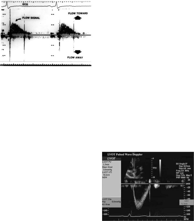
Doppler echo operates in two basic formats. Figure 10 depicts the CW method. An ultrasound signal is continuously transmitted into the heart while a second crystal (or array of crystals) in the transducer continually receives reflected signals. All red blood cells in the overlap region between the beam patterns of the transmit and receive crystals contribute to the calculated signal. The frequency
8 ECHOCARDIOGRAPHY AND DOPPLER ECHOCARDIOGRAPHY
Figure 11. Example of a continuous wave Doppler signal taken from a patient. Flow toward the transducer is a positive (upward) deflection from the baseline and flow away from the transducer is downward. ECG ¼ electrocardiogram signal.
content of this signal, combined with an electrocardiographic monitor lead, is then displayed on a strip chart similar to an M-mode echo (Fig. 11).
The advantage of the CW method is that it can detect a wide range of flow velocities encompassing every possible physiologic or pathologic flow state. The main disadvantage of the CW format is that the site of flow cannot be localized. To overcome the lack of localization of CW Doppler, a second format was developed called pulsed Doppler (PW). In this format, similar to B-mode echocardiographic imaging, brief bursts of ultrasound are transmitted at a given frequency followed by a silent interval (Fig. 12). Since the time it takes for a reflected burst of sound waves to return to the receiving crystal is directly related to the distance the reflecting structure is from the receiver, the position in the heart from which blood flow is sampled can be precisely controlled by limiting the time interval during which reflected ultrasound is received. This is known as range gating and allows the investigator to limit the area sampled to small portions of the heart or great vessel. There is a price to be paid for sample selectivity, however. The maximal detectable velocity PW Doppler is able to display is equal to one-half the pulse repetition frequency (frequently called the Nyquist limit). This reduces the number of situations in which flow velocity samples unambiguously display the flow phenomenon. A typical PW Doppler display shows flow both toward and away from the transducer (Fig. 13).
As one interrogates deeper structures progressively further from the transducer, the pulse repetition frequency must, of necessity, be decreased. As a result, the highest detectable velocity of the PW Doppler mode becomes progressively smaller. Due to attenuation, the sensitivity for detecting flow becomes progressively lower at greater distances from the transducer. Despite these limitations, selective sampling of blood flow allows interrogation of a wide array of cardiac structures in the heart.
When a measured flow has a velocity in a particular direction greater than the Nyquist limit, not all of the
Figure 12. Pulsed Doppler echocardiography. In place of a continuous stream of ultrasound, brief pulses are emitted similar to M-mode or 2D imaging. By acquiring reflected signal data over a limited time window following each pulse, reflections emanating only from a certain depth may be received. (From Feigenbaum H, Echocardiography (5th ed), Philadelphia, PA: Lea & Febiger; 1994, p 29, with permission from Lippincott Williams & Wilkins #.)
Figure 13. Example of a pulsed wave Doppler tracing. The study was recorded in duplex mode from the LVOT. The small upper insert shows the 2D image which guides positioning of the sample volume (arrow). The Doppler signal is shown below and has been traced by the sonographer using electronic analysis system. Data automatically detected from tracing the signal are shown on the left and include the peak velocity (PV) of flow and the integral of flow velocity (VTI) that can be used for calculations of cardiac output.
ECHOCARDIOGRAPHY AND DOPPLER ECHOCARDIOGRAPHY |
9 |
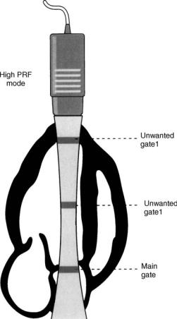
spectral envelope of the signal is visible. Indeed, the velocity estimates ‘‘wrap-around’’ to the other side of the velocity map and the flow appears to be going in the opposite direction. This phenomenon where large positives velocities are displayed as negative velocities is called aliasing. There are two strategies to mitigate or eliminate aliasing. The zero shift line (no velocity) may be moved upward or downward, effectively doubling the display range in the desired direction. This may be sufficient to ‘‘un-wrap’’ the aliased velocity and display it entirely in the appropriate direction. Some velocities may still be too high for this strategy to work. To display these higher velocities an alternative method called high pulse repetition frequency (high PRF) mode is employed. In this mode, sample volumes at multiples of the main interrogation sample volume are also interrogated. This is accomplished by sending out bursts of pulse packets at multiples of the burst rate necessary to sample at the desired depth. The system displays multiple sites from which the displayed signal might originate. While this creates some ambiguity in the exam, the anatomy displayed by the 2D exam usually allows a correct delineation as to which range gate is creating the signal (Fig. 14).
By itself, Doppler echo is a nonimaging technique that only produces flow patterns and audible tone patterns (since all Doppler shifts fall within the audible range). Phased array transducers, however, allow simultaneous display of both 2D images and Doppler in a mode called duplex Doppler echocardiography. By using this combination, the PW Doppler sample volume is displayed as an overlay on the 2D image and is moved to a precise area in the heart where the flow velocity is measured (Fig. 13). This combination provides both anatomic and physiologic information about the interrogated cardiac structure. Most commonly, Duplex mode is used with the PW wave format of Doppler echo. However, it is also possible to position the continuous wave beam anywhere in the 2D sector by superimposing the Doppler line of interrogation on top of the 2D image.
Just as changing from an M-mode echo to a 2D sector scan markedly increases the amount of spacial data simultaneously available to the clinician, Doppler information can be expanded from a single a PW wave sample volume or CW line to a full sector array. Color Doppler echocardiography displays blood flow within the heart or blood vessel as a sector plane of velocity information. By itself, a color flow scan imparts little information so the display is always combined with the 2D image as an overlay so blood flow may be instantly correlated with anatomic structures within the heart or vessel.
Color Doppler uses the same transmission principles as B-mode 2D imaging and PW Doppler. Brief transmit pulses of sound are steered along interrogation lines in a sector simultaneously with usual B-mode imaging pulses (Fig. 15). In place of just one pulse of sound, multiple pulses are transmitted. The multiple bursts of sound, typically 4–8 in number, are referred to as packets or ensembles of pulses. The first signal stores all reflected echoes along each scan line. Reflectors from subsequent pulses in the packet are received, stored, and rapidly compared to the previous packets. Reflected waves that are identical during each burst in the packet are canceled
Figure 14. Example of high PFR mode of pulsed Doppler. The signal is used for velocity detected at the main gate because pulse packets are sent out more frequently at multiples of the frequency needed to sample at the main gate. Information can also be acquired at other gates that are multiples of the main gate. While the Nyquist limit is higher due to a higher sampling rate some signal ambiguity may occur due to information acquired from the unwanted gates. (Reprinted from Zagzebski JA. Essentials of Ultrasound Physics. St. Louis: Mosby-Year Book Inc. copyright # 1996 with permission from Elsevier.)
out and designated as stationary. Reflected waves that progressively change from burst to burst are acquired and processed rapidly for calculation of the phase shift in the ultrasound carrier. Both direction and velocity of movement are proportional to this phase change. Estimates for the average velocity are assigned to a pixel location on the video display. The velocity is estimated by an auto correlator system. On the output display, velocity is typically displayed as brightness of a given color similar to B-mode gray scale with black meaning no motion and maximum brightness indicating the highest velocity detected. Two contrasting colors are used to display direction of flow, typically a red-orange group for flow toward the transducer and a blue group away from transducer. Since the amount of data processed is markedly greater than a typical B-Mode, maximum frame rates of sector scan displays tend to be much lower. This limitation is due both to the speed of sound and the multiple packets of ultrasound evaluated in each interrogation line. To maximize

10 ECHOCARDIOGRAPHY AND DOPPLER ECHOCARDIOGRAPHY
Figure 15. Diagram showing method of transmission of color flow Doppler ultrasound signals. Packets or ensembles of pulses represented by the open circles in the figure are sent out along some of the scan lines of the image. The reflected waves are analyzed in an autocorrelation circuit to allow display of the color flow image. (Reprinted from Zagzebski JA. Essentials of Ultrasound Physics. St. Louis: Mosby-Year Book Inc. copyright # 1996, with permission from Elsevier.)
time resolution, the color flow sector used to display data during a 2D echo may be considerably reduced in size compared to a usual 908 2D sector scan. Some systems can only display color flow data at relatively slow frame rates of 6–10 Hz. Recent innovations, in which there are multiple receive lines for each transmit line allow much higher frame rates giving excellent time resolution on some systems (7).
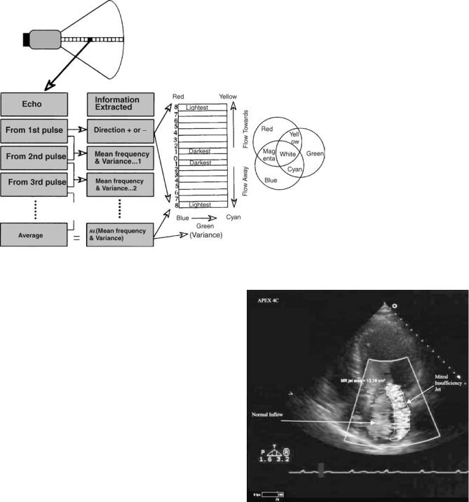
Clinically, precise measurement of flow velocity is usually obtained with PW or CW Doppler. Color is used to rapidly interrogate a sector for the presence or absence of blood flow during a given part of the cardiac cycle. Another important part of the color exam is a display of the type of flow present. Normal blood flow is laminar; abnormal blood flow caused by valve or blood vessel pathology is turbulent. The difference between laminar and turbulent flow is easily displayed by color Doppler. With laminar flow, the direction of flow is uniform and variation in velocity of adjacent pixels of interrogation is small. With turbulent flow, both parameters are highly variable. The auto correlation system analyzing color Doppler compares the variance in blood flow between different pixels. The display can be set to register a third color for variance such as green, or the clinician may look for a ‘‘mosaic’’ pattern of flow in which non uniform color velocities and directions are scattered through the sector areas of color interrogation (Figs. 16 and 17).
As with pulsed Doppler there is a Nyquist limit restriction on maximal velocity than can be displayed. The zero flow position line may be adjusted as with PW Doppler to maximize the velocity limit in a given direction. High PRF is not possible with color Doppler. The nature of the color display is such that aliasing results in a shift from one color sequence to the next. Thus, in some situations a high velocity shift can be detected due to a clear shift in color (e.g., from a red-orange sequence to a blue sequence). This phenomenon has been put to use clinically by purposely manipulating the velocity range of color display to force aliasing to occur. By doing this, isovelocity lines are displayed outlining a velocity border of flow in a particular direction and a particular velocity (8).
Thus far, all discussion of Doppler has been confined to interrogation and display of flow velocity. Alternate modes of interrogation are possible. One mode, called power Doppler (or energy display Doppler) assesses the amplitude of the Doppler signal rather than velocity. By evaluating amplitude in place of velocity, this display becomes proportional to the number of moving blood cells present in the interrogation field rather than the velocity. This application is particularly valuable for perfusion imaging when the amount of blood present in a given area is of primary interest (9).
ULTRASOUND SIGNAL PROCESSING, DISPLAY, AND MANAGEMENT
Once each set of the reflected ultrasound data returns to the transducer, it is processed and then transmitted to video display. The information is first processed by a scan converter, which assigns video data to a matrix array of picture elements, ‘‘pixels.’’ Several manipulations of the image are possible to reduce artifacts, enhance information in the display, and analyze the display quantitatively.
The concept of attenuation has been introduced earlier. In order to achieve a usable signal, the returning reflections must be amplified. The amplification can be done in multiple ways. Similar to a sound system, overall gain may be adjusted to increase or decrease the sensitivity of the received signal. More important, however, is the progressive loss of signal strength that occurs with reflections from deeper structures due to attenuation. To overcome this issue, ultrasound systems employ a variable gain circuit that selectively allows gain control at different depths. The applied gain is changed as a function of time (range) in the gain circuit, hence the term time gain compensation (TGC) is used to describe the process. This powerful tool can ‘‘normalize’’ the overall appearance of the image helping make much weaker returning echoes from great depth appear equal to near-field information (Fig. 18). The user also has slide pot control of gain as a function of depth. Some of this user-defined adjustment is applied as part of the TGC function or later as part of digital signal processing.
Manipulation of data prior to writing into the scan converter is called preprocessing. An important part of preprocessing is data compression. The raw data received by the transducer encompasses such a broad energy range
ECHOCARDIOGRAPHY AND DOPPLER ECHOCARDIOGRAPHY |
11 |
that it cannot be adequately shown on a video display. Therefore, the dynamic range of the signal is reduced to better fit visual display characteristics. Selective enhancement of certain parts of the data is possible to better display borders between structures. Finally, persistence may be added to the image. With this enhancement, a fraction of data from the previous video frames at each pixel location may be added and averaged together. This helps define weaker diffuse echo scatterers and may work well in a static organ. However, with the heart in constant motion, only modest amounts of persistence add value to the image. Too much persistence reduces motion resolution of the image.
Once the digital signal is registered in the scan converter, further image manipulation is possible. This is called postprocessing of the image. Information in digital memory has a 1:1 ratio between ultrasound signal amplitude and video brightness. Depending on the structure imaged, considerable information may not be discernible in the image. With postprocessing, the relationship of video brightness to signal strength can be altered, frequently to enhance weaker echos and suppress high amplitude echoes. This may result in a better appreciation of less echogenic structures such as myocardium and the edges of the myocardium. The gray scale image may be transformed to a pseudo-color display that adds color to video amplitude data. In certain circumstances this may allow differentiation of pathologic changes from normal. Selective magnification of the image is also possible (Fig. 19).
Figure 16. Diagram of color Doppler signal processing. At top, each box in the insonification line indicates a pulse of sound. A packet is made up of 4–8 pulses. The steps in the analysis cycle of a packet are shown in the ‘‘Echo’’ column and represent the comparison function of the autocorrelation system. From the first pulse the analysis determines the appropriate color representing direction. Comparisons between subsequent packets detect the velocity of blood flow. The brightness of the color selected corresponds to velocity. Comparisons of the variability of velocity are also done. Green is added proportional to the amount of variance. The final pixel color represents an average of the packet data for direction, velocity and variance. The right-hand column is the ‘‘color bar’’ that summarizes the type of map used, displays the range of color and brightness selected, and depicts how variance is shown. (From Sehgal CM, Principles of Ultrasound and Imaging and Doppler Ultrasound. In: Sutton, MG et al. editors: Textbook of Echocardiography and Doppler Ultrasound in Adults and Children (2nd ed). Oxford: Blackwell Science Publishing; 1996. p 29. Reprinted with permission of Blackwell Publishing, LTD. p 29)
Figure 17. Color Doppler (here shown in gray scale only) depicting mitral valve regurgitation. The large mosaic mitral insufficiency jet is caused by turbulent flow coming through the mitral valve. The turbulent flow area has been traced to measure its area. The more uniform flow in the left atrium is caused by normal flow in the chamber. It is of uniform color and of much lower velocity.
12 ECHOCARDIOGRAPHY AND DOPPLER ECHOCARDIOGRAPHY
Figure 18. Processing steps during transmission of sound data to the scan converter. Raw data emerges from the transducer (a) that is imaging two objects that produce specular border echoes at points 1, 2, 3, and 4 and scattered echoes in between. (b) Specular echo raw data. (c) Low noise amplification is applied. Both specular and scattered echoes are now shown. Relative signal strength declines with depth due to attenuation of the signal, making signal 4 weaker than signal 1 even though the material border interface at borders 1 and 4 are identical. (d) Time gain compensation is applied proportionally by depth to electronically amplify signals received progressively later after the pulse leaves the transducer. This helps equalize perceived signal strength (e). The signal is then rectified (f) and smoothed (g) before entering the scan converter. (h) The process is repeated several times per second, in this case all new data appears every 1/30 of a second. The end result is a ‘‘real-time’’ video display of the two structures. (From Sehgal SH, Principles of Ultrasound Imaging and Doppler Ultrasound. In: Sutton MG et al. editors. Textbook of Echocardio graphy and Doppler Ultrasound in Adults and Children. Oxford: Blackwell Science; 1996. p 11. Reprinted with permission of Blackwell Publishing, LTD.)
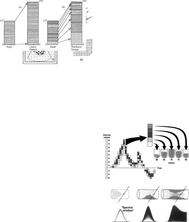
Signal processing of PW and CW Doppler data includes filtering and averaging, but the most important component of the analysis is the computation of the velocity estimates. The most commonly used method of analysis is the fast Fourier transform analyzer, which estimates the relative amplitude of various frequency components of the input signal. This system (Fig. 20) divides data up into discreet time segments of very short duration (1–5 ms). For each segment, amplitude estimates are made for each frequency that corresponds to different velocity components in the flow and the relative amplitude of each frequency is recorded on gray scale display. Laminar flow typically has a narrow, discrete velocity range on PW Doppler while turbulent flow may be composed of the entire velocity range. Differentiation of laminar from turbulent flow may help define normal from abnormal flow states. Similar analysis is used to display the CW Doppler signal. Color Doppler displays can be adjusted by using multiple types of display maps. Each manufacturer has basic and special proprietary maps available to enhance color flow data.
All Doppler data can be subjected to selective band pass filters. For conventional Doppler imaging, signals coming from immobile structures or very slow moving structures such as chamber walls and the pericardium, are effectively blanked out. The range of velocity filtered can be changed
Figure 19. B-mode post processing occurs in which signal input intensity varies from 0 to 127 units. On the left side of the figure a linear output is equally amplified, the signal intensity range is now 0–255. On the right, nonlinear amplification is applied. The output is manipulated to enhance or compress the relative video intensity of data. In this example high energy specular reflection video data is relatively compressed (high numbers) while low energy data (from scattered echoes and weak specular echoes) is enhanced. Thus relatively more of the video range is used for relatively weaker signals in the final product. This postprocessing is in addition to time gain compensation done during preprocessing. (From Sehgal SH. Principles of Ultrasound Imaging and Doppler Ultrasound, In: Sutton MG et al. editors: Textbook of Echocardiography and Doppler Ultrasound in Adults and Children. Oxford: Blackwell Science; 1996. p 12. Reprinted with permission of Blackwell Publishing, LTD.)
Figure 20. Upper panel Build-up of a spectral Doppler signal by Fast-Fourier analysis. The relative amplitude of the signal at each pixel location is assigned a level of gray. With laminar flow, the range of velocities is narrow resulting in a narrow window of displayed velocity. Lower panel As flow becomes more turbulent the range of velocities detected increases to the point that very turbulent signals may display all velocities. (Reprinted from Zagzebski JA. Essentials of Ultrasound Physics. St. Louis: Mosby-Year Book Inc. copyright # 1996, p 100,101, with permission from Elsevier.)
ECHOCARDIOGRAPHY AND DOPPLER ECHOCARDIOGRAPHY |
13 |
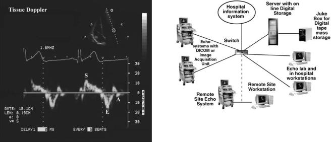
Figure 21. Example of tissue Doppler imaging. Duplex mode is used; the 2D image is shown in the upper insert. The sample volume has been placed outside the left ventricular cavity over the mitral valve annulus and is being used to detect movement of that structure. The three most commonly detected waveforms are shown: (S) systolic contraction wave, (E) early diastolic relaxation wave, and (A) atrial contraction wave.
for different clinical circumstances. In some situations, not all of the slower moving structures can be fully eliminated without losing valuable Doppler data, resulting in various types of artifact.
New techniques of Doppler analysis focus on analyzing wall motion with Doppler and displaying the data either in color or with Fourier transform analysis. In this setting, the band pass filters are set to eliminate all high velocity data from blood flow and only analyze very low velocity movement coming from the wall of the ventricles or other structures such as valve tissue. Analysis of tissue motion measures the velocity of wall movement at selected locations in the heart using the typical PW sample volume. Conventional strip chart display is used and velocity can be displayed to represent both the velocity of contraction and the velocity of relaxation (Fig. 21). Color Doppler uses the auto correlator system to calculate velocity of large segments of myocardium at once. Systems that record data at high color Doppler frame rates store sufficient information to allow selective time—velocity plots to be made at various locations of the cardiac chamber walls. Color Doppler may also be utilized to calculate strain and strain rate, another alternate display mode being investigated as a parameter of ventricular function (10,11).
Once the video signal processing is complete, it is displayed on a monitor. Until recently, most monitors were analogue and used standard NTSC video display modes. The composite (or RGB) signal was sent to a videocassette recorder for long-term storage and playback. The study could then be played on a standard video playback system for review and interpretation. Many laboratories continue to use this method of recording and storage of images.
Figure 22. Organization chart showing a digital echo image storage system. Images generated by the ultrasound systems in the hospital and remote sites are input via high speed links through a switch to the server. The server has on line digital storage and is linked to a jukebox mass storage device. From the server, data may be viewed at any workstation either in the hospital or remotely. The hospital information system is linked to the system. This can allow electronic ordering of studies, downloading of demographic data on patients and interface with the workstations. Typically, images are reviewed at a workstation; a report is composed and is electronically signed. The report is stored in the server but may also be sent to the Hospital Information System electronic record or put out on paper as a final report.
Recently, many echo laboratories have changed to digital image display and storage. In some labs, the ultrasound system directly records the study in digital format, storing data on a large hard disk in the ultrasound system. The data is then output, typically using a DICOM standard signal to a digital storage and display system. Other laboratories may attach an acquisition box to the ultrasound system that digitally records and transmits the RGB signal to a central image server.
A digital laboratory set up is shown in Fig. 22. It has several advantages over videotape. Image data is sent to a server and on to a digital mass storage device. Depending on the amount of digital storage and volume of studies in the lab, days to months of image data may be instantly available for review. More remote data is stored in a mass storage system (PACS system) on more inexpensive media such as digital tape. Data in this remote storage may be held online in a second ‘‘juke box’’ server or be fully off line in storage media that must be put back on line manually.
Digital systems link the entire lab together and are typically integrated with the hospital information system. Common studies may be organized by patient and displayed on multiple workstations within the laboratory, hospital, and at remote clinics. This is a marked improvement compared to having each study isolated to one videotape. The quality of the image is superior. High-speed fiber optic links allow virtually simultaneous image retrieval at remote sites. Lower speed links may need several minutes to transmit a full study. To reduce the amount of storage, studies are typically compressed. Compression ratios of 30:1 can be used without evidence of any significant image degradation.
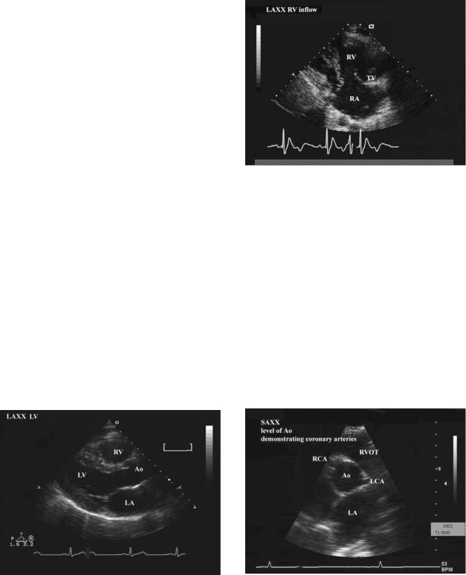
14 ECHOCARDIOGRAPHY AND DOPPLER ECHOCARDIOGRAPHY
THE ECHOCARDIOGRAPHIC EXAMINATION
The Transthoracic Exam
A full-featured cardiac ultrasound system is designed to allow the operator to perform an M-mode echo, 2D echo, CW Doppler, PW Doppler, color Doppler, and tissue Doppler examination. Except for the specialized CW Doppler transducer, the entire exam is usually performed with a broadband multipurpose transducer. Occasionally, a specialized transducer of a different frequency or beam focus must be utilized to interrogate certain types of suspected pathology. The examination is performed in a quiet, darkened room with the patient supine or lying in a left lateral position on a specialized exam bed. The transducer is covered with a coupling medium (gel-like substance) that allows a direct interface between the transducer head and the patient’s skin. If this coupling is broken the signal will be lost since ultrasound reflects strongly from tissue–air interfaces (Table 1). The transducer is then placed between the ribs, angled in the direction of the heart (ultrasound penetrates bone poorly and bone causes image artifacts), and adjusted until a satisfactory image is obtained (Fig. 2a). Electrodes for a single channel electrocardiogram are applied to the patient. The electrocardiogram signal is displayed continuously during the exam.
A standard examination begins in the left parasternal position (i.e., in the fourth and fifth rib interspaces just left of the sternum) (Fig. 2b). By orienting the 2D plane parallel to the long axis of the heart, an image of the proximal aorta, aortic valve, left atrium, mitral valve, and left ventricle can be obtained (Fig. 23). The standard M-mode echocardiographic views for dimension measurement are also obtained from this view (Fig. 6). Color Doppler is activated to examine flow near the mitral and aortic valves. By angulation from this position the tricuspid valve and portions of the right atrium and right ventricle are brought into view (Fig. 24). By rotation of the transducer 908 from the long axis, the parasternal short-axis view is obtained.
Figure 24. Parasternal long axis view angled toward the right ventricle. Right-sided structures are shown: right atrium (RA), right ventricle (RV) and tricuspid valve (TV).
By progressively changing the angle of the transducer it is possible to obtain a series of cross-sectional views through the left ventricle from near the apex to the base of the heart at the level of the origin of the great vessels (Figs. 25 and 26). In an optimal study, several cross-sections through the left ventricle, mitral valve, aortic valve, and to a lesser degree the tricuspid valve, pulmonic valve, and right ventricular outflow tract can be obtained. Since conventional 1D arrays yield only 2D images, only small slices of the heart are examined at any one time.
The transducer is then moved to the mid-left chest slightly below the left breast where the apex of the heart touches the chest wall (Fig. 2). The 2D transducer is then angled along the long axis toward the base of the heart. The result is a simultaneous display of all four chambers of the heart and the mitral and tricuspid valves (Fig. 27). No M- mode views are taken from this position. Using duplex
Figure 23. Parasternal long axis view of the heart (LAXX) similar to orientation shown in Fig. 6. Abbreviations are as follows: aorta (Ao), left ventricle (LV), left atrium (LA), and right ventricle (RV). This is a 2D image.
Figure 25. Parasternal short axis view at the level of the great vessels. Shown is the aorta (Ao), a portion of the left atrium (LA), the origin of the left (LCA), and right (RCA) coronary arteries, and a part of the right ventricular outflow tract.
ECHOCARDIOGRAPHY AND DOPPLER ECHOCARDIOGRAPHY |
15 |
Figure 26. Short axis orientation at the transducer (SAXX) showing a cross-sectional view of the left ventricle (LV). The muscle appears as a ring. The septum (IVS) separates the LV from the right ventricle (RV).
mode, PW Doppler samples of blood flow are taken to show the forward flow signal across the mitral and tricuspid valves (Fig. 28). By further anterior angulation, the left ventricular outflow tract and aortic valve are imaged (Fig. 29) and forward flow velocities are sampled at each site. The 2D image allows precise positioning of the Doppler sample volume. By rotation of the transducer, further selective portions of the walls of the left ventricle are obtained (Fig. 30). Color Doppler is then used to sample blood flow across each heart valve, screening for abnormal turbulent flow, particularly related to valve insufficiency (leakage during valve closure). The transducer is then moved to a location just below the sternum (Fig. 2b) and aimed up toward the heart where the right atrium and atrial septum can be further interrogated, along with partial views of the other chambers (Fig. 31). In some
Figure 28. By using the same transducer orientation as Fig. 27, several other types of data are obtained. In this case, the system has been switched to Duplex mode. The 2D echo is used as a guide to position the mitral sample volume (small upper image). Flow is obtained across the mitral valve (MV) with waveforms for early (E), and atrial (A) diastolic flow shown.
patients, cross-sectional views equivalent to the short-axis view may be obtained.
However, this view in most patients is less useful because the heart is further from the transducer causing reduced resolution and increased attenuation of the echo signals. Finally, the heart may be imaged from the suprasternal approach (Fig. 2b), which generally will allow a view of the ascending aorta and aortic arch (Fig. 32).
Figure 27. The transducer is placed in the apical position. The view shown is the apical ‘‘four chamber’’ view since all four chambers of the heart can be imaged simultaneously. Abbreviations are as follows: left ventricle (LV), left atrium (LA), right atrium (RA), and right ventricle (RV).
Figure 29. From the view shown in Fig. 27, the transducer has been tilted slightly to show the outflow region of the left ventricle (LV) where blood is ejected toward the aorta (Ao). Abbreviations are as follows: left atrium (LA), right atrium (RA), and right ventricle (RV).
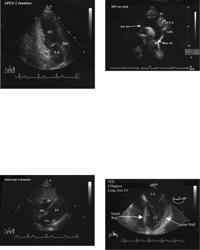
16 ECHOCARDIOGRAPHY AND DOPPLER ECHOCARDIOGRAPHY
Figure 30. From the position shown in Fig. 27, the transducer is rotated to show a different perspective from the apical view. The ‘‘two-chamber’’ view shows only the left-sided chambers and the mitral valve (MV) that controls flow between these two chambers. Abbreviations are as follows: left ventricle (LV) and left atrium (LA).
The Transesophageal Exam
About 3–10% of hospital-based echocardiograms are performed using a specialized transesophageal (TEE) device. The ultrasound transducer, smaller but otherwise of virtually equal capability to the transthoracic device, is attached to the end of an endoscope. The patient is prepared using a topical anesthetic agent in the mouth and pharynx to eliminate the gag reflex and given conscious sedation to increase patient comfort. Patient status is monitored by a nurse, the ultrasound system operated by a sonographer
Figure 32. The transducer is positioned at the suprasternal notch (see Fig. 2b). A portion of the aorta (Asc Ao and Dsc Ao) is visible along with the origins of three branches coming off of this structure: innominate artery (IA), left common carotid artery (LCCA) and left subclavian (LSC).
and the transducer inserted by a physician who personally performs the exam. As the transducer is passed down in the esophagus, multiple imaging planes are obtained. These planes are obtained by a combination of movement of the transducer to different levels of the esophagus, changing the angle of the transducer and controlling the transducer head. Originally, the transducer was fixed in one location on the endoscope. Virtually all devices now made allow the operator to rotate the transducer through a 1808 arc markedly increasing the number of imaging planes in the exam (Figs. 33–35). Using this method multiple views of structures in both a long and short axis configuration are possible. The transducer may also be passed into the stomach where additional views are possible.
Figure 31. The transducer is moved to the subcostal position (see Fig. 2b). Portions of all four chambers are visible. Abbreviations are as follows: left atrium (LA), left ventricle (LV), right atrium (RA), and right ventricle (RV).
Figure 33. Image generated by a transducer placed in the esophagus. Abbreviations are as follows: left ventricle (LV) and left atrium (LA).
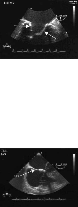
ECHOCARDIOGRAPHY AND DOPPLER ECHOCARDIOGRAPHY |
17 |
Figure 34. Image from a transesophageal transducer. This is a magnified view of the mitral valve leaflets (arrows).
The exam is performed in a similar fashion to the transthoracic exam in that multiple views of cardiac chambers and valves are taken in an organized series of views to achieve a complete examination of the heart. Many planes are similar to the transthoracic exam except for location of the transducer. Other views are unique to the TEE exam and may be the clinical reason the exam was performed. Once the exam is complete, the transducer is removed, and the patient is monitored until recovered from the sedation and topical anesthesia.
The Intracardiac Exam
During specialized procedures it may be valuable to examine the heart from inside. This is usually done during specialized sterile cardiac procedures when a transthoracic transducer would be cumbersome or impossible to use and a TEE also would be impractical.
Figure 35. Image from a transesophageal transducer. The septal structure (IAS) that separates the two atrial chambers is shown (arrow).
A catheter with a miniaturized transducer is passed under fluoroscopic guidance up large central veins from the groin to the right side of the heart. For most applications, the device may be placed in the right atrium, or infrequently, in the right ventricle. The transducer is a miniature phased array device that can provide 2D and Doppler information. In most cases, the clinical diagnosis is already known and the patient is undergoing a specialized cardiac procedure in the catheterization laboratory to close a congenital defect or monitor radio frequency ablation during a complex electrophysiologic procedure, attempting to eliminate a cardiac rhythm disorder. The device contains controls that allow change of angle in four directions. This, combined with positional placement of the catheter in different parts of the cardiac chambers, allows several different anatomic views of cardiac structures (Fig. 36).
The Stress Echo Exam
Combining a transthoracic echo with a stress test was first attempted in the 1980s, became widely available in the mid-1990s, and is now a widely utilized test for diagnosis of coronary artery disease. The echo exam itself is purposely brief, usually confined to 4–6 2D views.
A patient having a stress echo is brought to a specialized stress lab that contains an ultrasound system set up to acquire stress images, an exam table, and a stress system that most commonly consists of a computerized electrocardiography system that runs a motorized treadmill (Fig. 37). The patient is connected to the 12-lead electrocardiogram stress system and a baseline electrocardiogram is obtained. The baseline echo is next performed, recording 2D views (Fig. 38). Then the stress test is begun. It can be performed in two different formats:
1.Exercise: If the patient is able to walk on a treadmill (or in some labs, pedal a bike), a standard maximal exercise test is performed until maximum effort has been achieved. Immediately upon completion of exercise, the patient is moved back to the echo exam table and repeat images are obtained within 1–2 min of completion of exercise.
2.Pharmacologic stimulation: If the patient is unable to exercise, an alternative is stimulation of the heart with an intravenous drug that simulates exercise. Most commonly, this is dobutamine, which is given, in progressively higher doses in 3–5 min stages. The patient remains on the exam table the entire time, connected to the electrocardiographic stress system. 2D echo images are obtained; at baseline, low dose, intermediate dose, and peak dose of drug infusion during the exam.
In both types of tests, clinical images are recorded and then displayed so that pretest and posttest data can be examined side by side. Comparisons of cardiac function are carefully made between the prestress and poststress images. The test relies on perceived changes in mechanical motion of different anatomic segments of the heart. Both inward movement of heart muscle and thickening of the walls of the ventricles are carefully evaluated. The normal

18 ECHOCARDIOGRAPHY AND DOPPLER ECHOCARDIOGRAPHY
Figure 36. (a) Image of the atrial septum in a patient with an atrial septal defect (arrow). This image was taken with an intracardiac transducer placed in the right atrium (RA). The image is of similar quality to that seen in Fig. 35. (b) Image of same structure as (a) demonstrating color flow capabilities at the intracardiac transducer. Color Doppler (seen in gray scale) confirms the structure is a hole with blood passing through the hole (ASD shunt). (c) Image taken from same position as (a) and (b). The atrial septal defect has been closed with an occluder device (arrow). Doppler was used (not shown) to confirm that no blood could pass through the previously documented hole.
Figure 37. Typical set-up of a laboratory to perform stress echocardiograms. Shown are the echocardiographic examination table (ET), the treadmill (T), the treadmill computer control system (TC), and the ultrasound system (US).
heart responds by augmenting inward motion and wall thickening in all regions. If blood supply to a given segment is not adequate, mechanical motion and wall thickening either fails to improve or deteriorates in that segment, but improves in other segments. This change defines an abnormal response on a stress echo (Fig. 38). The location and extent of abnormal changes in wall motion and thickening are reported in a semiquantitative manner. In addition, the electrocardiogram response to stress is also compared with the baseline exam and reported along with patient symptoms and exercise capacity.
Figure 38. Quad screen format of view obtained from a stress echocardiography examination. Four views are displayed simultaneously, and the particular views shown can be changed to accommodate direct comparison of pre- (images on the left) and posttest images on the right views of the same part of the heart as shown in the example. The arrow indicates an area of the heart that failed to respond normally.
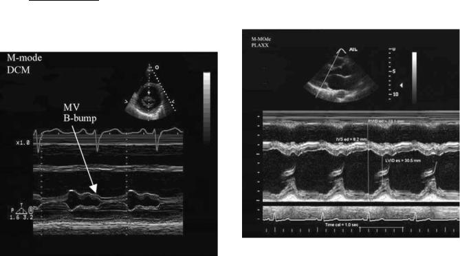
ECHOCARDIOGRAPHY AND DOPPLER ECHOCARDIOGRAPHY |
19 |
CLINICAL USES OF ECHOCARDIOGRAPHY
M-Mode Echocardiography
The M-mode echo was the original cardiac exam and for years was the dominant cardiac ultrasound study performed. The 2D echo has superseded M-mode echo as the primary examination technique and in most circumstances is superior. However, many laboratories continue to perform at least a limited M-mode exam because dimension measurements are well standardized. In addition, due to its high sampling rate, M-mode echo is superior to 2D echo for timing of events within the cardiac cycle and for recording simultaneously, with other physiologic measurements such as phonocardiograms and pulse tracings. Certain movement patterns of heart valves and chamber walls are only detected by M-mode, thus providing unique diagnostic information (Fig. 39).
Most M-mode echo data is obtained from multiple different ‘‘ice pick’’ views, all obtained from the parasternal position (Fig. 7). The 2D image is used to direct the cursor position of these views. The first view angles through a small portion of the right ventricle, the ventricular septum, the left ventricular chamber, the posterior wall of the left ventricle, and the pericardium. From this view, left ventricular wall thickness and the shortaxis dimensions of this chamber can be measured. By calculating the change in dimension between end diastole (at the beginning of ejection) and end systole (at the end of ejection), the fractional shortening can be measured using the equation:
LVEDD LVESD ¼ fractional shortening
LVEDD
where LVEDD is the left ventricular end diastolic dimension and LVESD is the left ventricular end systolic dimen-
sion. This measurement estimates left ventricular function (Fig. 40). Dimension measurements give a relatively precise estimate of left ventricular chamber size to calculate whether the ventricle is inappropriately enlarged. In a similar manner wall thickness measurements can be utilized to determine if the chamber walls are inappropriately thick (left ventricular hypertrophy), asymmetrically thickened (hypertrophic cardiomyopathy), or inappropriately thin (following a myocardial infarction).
The second ice pick view passes through the right ventricle, septum, mitral valve leaflets, and posterior wall. This view is used primarily to evaluate motion of the mitral valve. Certain types of mitral valve disease alter the pattern of motion of this valve (Fig. 39). Other abnormal patterns of leaflet motion may indicate dysfunction elsewhere in the left ventricle.
The third ice pick view passes the echo beam through the right ventricle, aortic valve, and left atrium. From this view, analogous to the mitral valve, the pattern of aortic valve motion will change in characteristic ways allowing the diagnosis of primary aortic valve disease or diseases that cause secondary aortic valve motion changes. Also, from this view the diameter of the left atrium is measured and whether this structure is of normal size or enlarged can be of considerable importance in several circumstances. Other views are possible, but rarely used.
Measurements taken from M-mode may be performed during the exam by the sonographer. Usually, the scrolling M-mode video display is saved in digital memory on the system. The saved data is then reviewed until the best depiction of the various views discussed above is displayed. The sonographer then uses electronic calipers, automatically
Figure 39. Example of an M-mode echocardiogram of the mitral vale showing abnormal motion, in this case a ‘‘B-bump’’ indicating delayed closure of the valve. DCM ¼ dilated cardiomyopathy.
Figure 40. Example of an M-mode echocardiogram of the left ventricle. The typical measurements of wall thickness (IVSed and LVPWed) and chamber dimensions (RVIDed, LVIDed and LVIDes) are shown. Several calculated parameters are possible from these values.
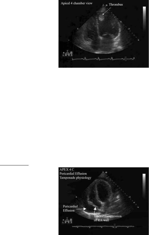
20 ECHOCARDIOGRAPHY AND DOPPLER ECHOCARDIOGRAPHY
calibrated by the system, to record dimension measurements (Fig. 40). Basic measures are made and formulas for derived data such as the % FS are automatically calculated. Measurements can also be made ‘‘off line’’ using special workstations that display the video information at the time the study is interpreted by the physician.
Two-Dimensional Echocardiography
The 2D exam gives information about all four cardiac chambers and all four cardiac valves. It also serves as the reference point for positioning all Doppler sample volumes and the color Doppler exam. The heart is imaged from multiple positions, which not only improves the chance of useful information being obtained, but also allows better characterization of a given structure because the structure is seen in several perspectives. The primary role of a 2D echo is to characterize the size of the left and right ventricles as normal or enlarged, and if enlarged, estimate the severity of the problem. Second, the 2D exam evaluates pump function of the two ventricles. Function is characterized globally (i.e., total ventricular performance) or regionally (i.e., performance of individual parts of each ventricle). Some types of disease affect muscle function relatively equally throughout the chambers. Other forms of disease, most notably coronary artery atherosclerosis, which selectively changes blood supply to various parts of the heart, cause regional changes in function. In this disease, some portions of the heart may function normally while other areas change to fibrous scar and decrease or stop moving entirely. Global function of the left ventricle can be characterized quantitatively. The most common measurements of function use calculations of volume during the cardiac cycle. This is quantified when the heart is filled maximally just before a beat begins and minimally just after ejection of blood has been completed. The volume calculations are used to determine of ejection fraction. The equation is
Ejection fraction ¼ LVEDV LVESV 100
LVEDV
Figure 41. Example of detection of a blood clot (thrombus) in the left ventricular chamber.
Doppler Echocardiography
While the 2D echo has considerably expanded the ability to characterize abnormalities of the four heart valves, it has not been possible to obtain direct hemodynamic information about valve abnormalities by imaging alone. Doppler imaging provides direct measurement of hemodynamic information.
By using Doppler, six basic types of information can be obtained about blood flow across a particular region:
1.The direction of the blood flow.
2.The time during the cardiac cycle during which blood flow occurs.
3.The velocity of the blood flow.
4.The time the peak velocity occurs.
5.The rate at which velocity changes.
where LVEDV ¼ left ventricular end diastolic volume and LVESV ¼ left ventricular end systolic volume.
The 2D echo is sensitive for detecting abnormalities within the chambers, such as blood clots or vegetations (infectious material attached to valves). Abnormalities surrounding the heart, such as pericardial effusions (fluid surrounding the heart), metastatic spread of tumors to the heart and pericardium, and abnormalities contiguous to the heart in the mediastinum or great vessels can be readily imaged. Most of this information is descriptive in nature (Figs. 41 and 42).
The ability to directly and precisely make measurements from 2D echo views for quantitative measurements of dimensions, areas, and volumes is built into the ultrasound system and is typically done by the sonographer during the exam in a similar fashion to M-mode. Further measurements may be performed off line on dedicated analysis computers. Many parts of the interpretation of the exam, however, remain primarily descriptive and are usually estimated by expert readers.
Figure 42. Example of a patient with fluid surrounding the heart. The dark area surrounding the heart (pericardial effusion) is shown. In this case, increased pressure caused by the effusion compresses part of the right atrium (RA).
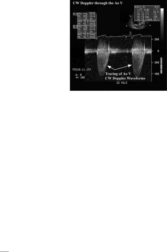
ECHOCARDIOGRAPHY AND DOPPLER ECHOCARDIOGRAPHY |
21 |
6.The pressure drop or gradient across a particular valve or anatomic structure.
Data about pressure gradients is derived from the velocity measurement using the Bernoulli equation:
|
|
|
2 dv |
|
||
P1 P2 |
¼ 1=2rðV22 V12 |
Þ |
þ r ð1 |
|
ds |
þ R ðvÞ |
dt |
||||||
|
| {z } |
acceleration |
| {z } |
|||
|
Convective |
|
| {z } |
Viscous |
||
|
acceleration |
|
Flow |
friction |
||
|
|
|
|
|
||
where Pl P2 is the pressure drop across the structure V2 and V1 being blood flow velocity on either side of the structure, and r is the mass density of blood (1.06 103 kg/m3). For applications in the heart, the contributions by the flow acceleration and viscous friction terms can be ignored. In addition, V1 is generally much less than V2 (thus, V1 can usually be ignored), and r is a constant for the mass density of blood (6). Combining all these changes together results in the final ‘‘simplified’’ form of the Bernoulli equation:
P1 P2 ¼ 4 V2
Cardiac Output. When the heart rate, blood flow velocity integral, and cross-sectional area of the region across which the blood flow is measured are known, cardiac output can be estimated using the following equation:
CO ¼ A V HR
where CO is the cardiac output, A is the cross-sectional area, V is the integrated blood flow velocity, and HR is the heart rate.
The Character of the Blood Flow. The differentiation between laminar and turbulent blood flow can be made by observation of the spectral pattern. In general, laminar flow (all recorded velocities similar) occurs across normal cardiac structures of the heart, while disturbed or turbulent flow (multiple velocities detected) occurs across diseased or congenitally abnormal cardiac structures (Fig. 20).
Doppler is most valuable in patients with valvular heart disease and congenital heart disease. In the case of valve stenosis (abnormal obstruction to flow), use of Doppler echocardiography allows quantification of the pressure gradient across the valve (Fig. 43). Using the continuity principle, which states that the product of cross-sectional area and flow velocity must be constant at multiple locations in the heart, it is possible to solve for the severity of valve stenosis. The equation may be written as noted and then manipulated to solve for the area at the stenotic valve (A2).
A1V1 ¼ A2V2
A1V1 ¼ A2
V2
For valvular insufficiency, Doppler echocardiography is most useful when the color Doppler format is used in
Figure 43. Example of a continuous wave Doppler signal through the aortic valve (AoV). Two tracings are shown along with measurement technique also demonstrated.
conjunction with 2D echo. Since an insufficient valve (i.e., a valve that allows backward leakage of blood when closed) produces turbulent flow in the chamber behind the valve, color Doppler immediately detects its presence. The extent to which turbulent flow can be detected is then graded on a semiquantitative basis to characterize the amount of valve insufficiency (Fig. 17). Since only 2D are interrogated at any given time, the best results are obtained when Doppler sampling is done from more than one view.
In patients with congenital heart disease, Doppler echocardiography allows the tracing of flow direction and velocity across anatomic abnormalities, such as holes between various cardiac chambers (i.e., atrial or ventricular septal defects). It can also display gradients across congenitally malformed valves and great vessels and also determine the direction and rate of flow through anatomically mal positioned chambers and great vessels.
In addition to direct interrogation of heart valves for detection of primary valve disease, Doppler flow sampling is used to evaluate changes in flow across normal valves that may indicate additional pathology. For example, the systolic blood pressure in the lungs (pulmonary artery pressure) may be estimated by quantifying the velocity of flow of an insufficiency jet across the tricuspid valve (another application of the Bernoulli equation). This calculated value, when added to the estimated central venous pressure (obtained in a different part of the exam) gives an excellent estimate of pulmonary artery pressure.
A second important measurement involves characterizing the way the left ventricle fills itself after ejecting blood into the aorta. There is a well-described set of changes in the pattern of flow across the mitral valve, changes in flow into the left atrium from the pulmonary veins and changes in the outward movement in the muscle itself characterized
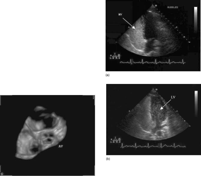
22 ECHOCARDIOGRAPHY AND DOPPLER ECHOCARDIOGRAPHY
by tissue Doppler that can help categorize the severity of changes in filling of the left ventricle.
SPECIALIZED CLINICAL DATA
Transesophageal Echocardiography
The TEE exam is used when a transthoracic exam either cannot be performed or gives inadequate information. One limitation of echo is the great degree of variability in image quality from patient to patient. In some circumstances, particularly in intensive care units, the TEE exam may provide superior image quality since its image quality is not dependent on patient position or interfered with by the presence of bandages, rib interfaces, air or other patient dependent changes. Similarly, during open heart surgery a TEE is routinely used to assess cardiac function preand postintervention and preand postheart valve replacement or repair. Since the TEE probe is in the esophagus, outside of the surgeon’s sterile field images are obtained even when the patient’s chest is open. This capability allows the surgeon to evaluate the consequences of, for example, a surgical repair of a heart valve, when the heart has been restarted, but before the chest is sutured closed. The TEE exam also visualizes parts of the heart not seen by any transthoracic view. A particular example of this is the left atrial appendage, a part of the left atrium. This structure sometimes develops blood clots that can only be visualized by TEE.
Three-Dimensional Reconstruction
While the 2D exam displays considerable data about spatial relationships between structures and quantification of volume, there is still considerable ambiguity in many circumstances. One way to further enhance the exam is to use 3D reconstruction.
Its use has been a significant challenge. All early methods developed computerized routines that characterized the movement of the transthoracic transducer in space. Images were acquired sequentially and then reconstructed first using geometric formulae and later using more flexible algorithms without geometric assumptions. The data, while shown to be useful for both adding new insight into several cardiac diseases and improving quantitation, did not achieve practical acceptance due to the considerable operator time and effort required to obtain just one image (12).
Recently innovations in image processing and transducer design have produced 3D renditions of relatively small sections of the heart in real time. Use remains limited at present but further development is expected to make 3D imaging a practical reality on standard ultrasound systems (Fig. 44).
Figure 44. Example of on-line 3D reconstruction. The heart is imaged at the level of the aortic valve where all three leaflets are shown.
Figure 45. (a) Example of injection of agitated saline into systemic veins. The contrast moves into the right atrium (RA) and right ventricle (RV), causing transient full opacification. The leftsided chambers are free of contrast. (b) Similar to (a). However, some of the contrast bubbles have crossed to the left ventricle (LV), proving a communication exists between the right and left sides of the heart.
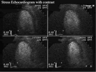
ECHOCARDIOGRAPHY AND DOPPLER ECHOCARDIOGRAPHY |
23 |
Figure 46. Example of contrast use to improve visualization of the walls of the left ventricle. The contrast agent used in this case is a gas-filled microbubble that fills the left ventricle during a stress test. The entire chamber is white with full contrast enhancement.
Contrast Imaging
Contrast agents are combined with certain 2D echo exams to enhance the amount of diagnostic information available on the exam, or improve the quality of the exam.
There are two types of contrast agents. One type is made from normal saline solution. An assistant generates the contrast for injection during regular 2D imaging. Typically 0.5 mL of air is added to a 10 mL syringe of saline and vigorously hand agitated between 2 syringes for about 15 s. This agitation causes production of several million small bubbles. The bubbles are too large to pass through capillaries, thus when injected into a vein, they are all filtered out by the passage of venous blood through the lungs. Thus when injected into a normal heart, saline contrast passes into the right atrium and right ventricle, produces a transient intense response and disappears, not making it to the left ventricle. This property makes saline injection ideal for detecting an abnormal hole, or shunt passage across the atrial septum or ventricular septum. When a communication of this type is present bubbles cross directly from the right side to the left side of the heart. This is an extremely sensitive method for making this diagnosis (Fig. 45).
A second type of contrast agent, developed and now commercially marketed, is a gas filled microbubble smaller than a red blood cell. This type of agent, made from perfluorocarbons covered by an albumen or lipid shell, when intravenously injected passes through the lungs and opacifies the left side of the heart as well as the right side. The bubbles are gradually destroyed by ultrasound and blood pressure, lasting for several minutes in ideal circumstances. When combined with harmonic imaging these contrast agents markedly improve the quality of the 2D image, particularly for the evaluation of left ventricular wall motion (Fig. 46). The contrast agent markedly enhances the border between blood and the chamber wall. Use of these agents is variable among laboratories, but its use substantially decreases the number of nondiagnostic
studies. Still under investigation is whether these same contrast agents can be used for evaluation of blood flow within the heart muscle. This information could be of particular value for patients with coronary artery disease either during acute episodes of ischemia when a new coronary stenosis is suspected or as an enhancement to the stress echocardiogram (13).
BIBLIOGRAPHY
Cited References
1.Edler I, Hertz CH. The use of ultrasonic reflectoscope for the continuous recording of the movements of heart walls. Kungl Fysiografiska sa¨llskapets I lund forhandlingar 1954;24(5):1– 19.
2.Zagzebski JA. Physics of Diagnostic Ultrasound. In: Rowland J, editor. Essentials of Ultrasound Physics. St. Louis: Mosby; 1996. p 1–18.
3.Hancock J, Dittrich H, Jewitt DE, Monaghan MJ. Evaluation of myocardial, hepatic and renal perfusion in a variety of clinical conditions using an intravenous ultrasound contrast agent (Optison) and second harmonic imaging. Heart 1999;81:636–641.
4.Spencer KT, Bednarz J, Rafter PG, Korcarz C, Lang RM. Use of harmonic imaging without echocardiographic contrast to improve two-dimensional image quality. Am J Cardiol 1998; 82:794–799.
5.Kisslo J, VonRamm OT, Thurstone FL. Cardiac imaging using a phased array ultrasound system II: clinical technique and application. Circulation 1976;53:262–267.
6.Nishimura RA, Miller FA, Callahan MI, Benassl RC, Seward JB, Tajik AJ. Doppler echocardiography: Theory, instrumentation, technique and application. Mayo Clinic Proc 1985;60:321–343.
7.Omoto R, Kasai C. Physics and instrumentation of Doppler color mapping. Echocardiography 1987;4:467–483.
8.Vandervoort PM, Rivera JM, Mele D, Palacios IF, Dinsmore RE, Weyman AE, Levine RA, Thomas JD. Application of color Doppler flow mapping to calculate effective regurgitant orifice area. Circulation 1993;88:1150–1156.
9.Burns PN. Instrumentation for contrast echocardiography. Echocardiography 2002;19:241–258.
10.Sade LE, Severyn DA, Kanzaki H, Dohi K, Gorcsan J. Second generation tissue Doppler with angle corrected color codes wall displacement for quantitative assessment of regional left ventricular function. Am J Cardiol 2003;92:554–560.
11.Urhelm S, Edvardson T, Torpi H, Angelsen B, Smiseth O. Myocardial strain by Doppler echocardiography: Validation of a new method to quantify regional myocardial function. Circulation 2000;102:1158–1164.
12.Mele D, Levine RA. Quantitation of ventricular size and function: Principles and accuracy of transthoracic rotational scanning. Echocardiography 2000;17:749–755.
13.Porter TR, Cwajg J. Myocardial contrast imaging: A new gold standard for perfusion imaging. Echocardiography 2001; 18:79–87.
Reading List
Anderson B. Echocardiography: The Normal Examination and Echocardiographic Measurements. Brisbane: Fergies; 2000.
Goldberg BB. Ultrasound Contrast Agents. St. Louis: Mosby Year Book; 1997.
Feigenbaum H. Echocardiography. 5th ed. Philadelphia: Lea & Febiger; 1994.