

- •VOLUME 3
- •CONTRIBUTOR LIST
- •PREFACE
- •LIST OF ARTICLES
- •ABBREVIATIONS AND ACRONYMS
- •CONVERSION FACTORS AND UNIT SYMBOLS
- •EDUCATION, COMPUTERS IN.
- •ELECTROANALGESIA, SYSTEMIC
- •ELECTROCARDIOGRAPHY, COMPUTERS IN
- •ELECTROCONVULSIVE THERAPHY
- •ELECTRODES.
- •ELECTROENCEPHALOGRAPHY
- •ELECTROGASTROGRAM
- •ELECTROMAGNETIC FLOWMETER.
- •ELECTROMYOGRAPHY
- •ELECTRON MICROSCOPY.
- •ELECTRONEUROGRAPHY
- •ELECTROPHORESIS
- •ELECTROPHYSIOLOGY
- •ELECTRORETINOGRAPHY
- •ELECTROSHOCK THERAPY.
- •ELECTROSTIMULATION OF SPINAL CORD.
- •ELECTROSURGICAL UNIT (ESU)
- •EMERGENCY MEDICAL CARE.
- •ENDOSCOPES
- •ENGINEERED TISSUE
- •ENVIRONMENTAL CONTROL
- •EQUIPMENT ACQUISITION
- •EQUIPMENT MAINTENANCE, BIOMEDICAL
- •ERGONOMICS.
- •ESOPHAGEAL MANOMETRY
- •EVENT-RELATED POTENTIALS.
- •EVOKED POTENTIALS
- •EXERCISE FITNESS, BIOMECHANICS OF.
- •EXERCISE, THERAPEUTIC.
- •EXERCISE STRESS TESTING
- •EYE MOVEMENT, MEASUREMENT TECHNIQUES FOR
- •FETAL MONITORING
- •FETAL SURGERY.
- •FEVER THERAPY.
- •FIBER OPTICS IN MEDICINE
- •FICK TECHNIQUE.
- •FITNESS TECHNOLOGY.
- •FIXATION OF ORTHOPEDIC PROSTHESES.
- •FLAME ATOMIC EMISSON SPECTROMETRY AND ATOMIC ABSORPTION SPECTROMETRY
- •FLAME PHOTOMETRY.
- •FLOWMETERS
- •FLOWMETERS, RESPIRATORY.
- •FLUORESCENCE MEASUREMENTS
- •FLUORESCENCE MICROSCOPY.
- •FLUORESCENCE SPECTROSCOPY.
- •FLUORIMETRY.
- •FRACTURE, ELECTRICAL TREATMENT OF.
- •FUNCTIONAL ELECTRICAL STIMULATION
- •GAMMA CAMERA.
- •GAMMA KNIFE
- •GAS AND VACUUM SYSTEMS, CENTRALLY PIPED MEDICAL
- •GAS EXCHANGE.
- •GASTROINTESTINAL HEMORRHAGE
- •GEL FILTRATION CHROMATOGRAPHY.
- •GLUCOSE SENSORS
- •HBO THERAPY.
- •HEARING IMPAIRMENT.
- •HEART RATE, FETAL, MONITORING OF.
- •HEART VALVE PROSTHESES
- •HEART VALVE PROSTHESES, IN VITRO FLOW DYNAMICS OF
- •HEART VALVES, PROSTHETIC
- •HEART VIBRATION.
- •HEART, ARTIFICIAL
- •HEART–LUNG MACHINES
- •HEAT AND COLD, THERAPEUTIC
- •HEAVY ION RADIOTHERAPY.
- •HEMODYNAMICS
- •HEMODYNAMIC MONITORING.
- •HIGH FREQUENCY VENTILATION
- •HIP JOINTS, ARTIFICIAL
- •HIP REPLACEMENT, TOTAL.
- •HOLTER MONITORING.
- •HOME HEALTH CARE DEVICES
- •HOSPITAL SAFETY PROGRAM.
- •HUMAN FACTORS IN MEDICAL DEVICES
- •HUMAN SPINE, BIOMECHANICS OF
47.Gluckman PD, Wyatt JS, Azzopardi D, Ballard R, Edwards AD, et al. Selective head cooling with mild systemic hypothermia after neonatal encephalopathy: A multicentre randomised trial. Lancet 2005;365:663–670.
48.Qui WS, Liu WG, Shen H, Wang WM, Hang ZL, Jiang SJ, Yang XZ. Therapeutic effect of mild hypothermia on severe traumatic head injury. Chin J Traumatol 2005;8:27–32.
49.Dyson M, Moodley S, Verjee L, Verling W, Weinman J, Wilson P. Wound healing assessment using 20 MHz ultrasound and photography. Skin Res Technol 2003;9: 116–121.
HEAVY ION RADIOTHERAPY. See RADIOTHERAPY,
HEAVY ION.
HEMODYNAMICS
PATRICK SEGERS
PASCAL VERDONCK
Ghent University
Belgium
INTRODUCTION
‘‘Arterial blood pressure and flow result from the interaction of the heart and the arterial system. Both subsystems should be considered for a complete hemodynamic profile and a better diagnosis of the patient’s disease’’. This statement seems common sense, and a natural engineering approach of the cardiovascular system, but is hardly applied in clinical practice, where clinicians have to deal with limitations imposed by the clinical environment and ethical and economical considerations. The result is that the interpretation of arterial blood pressure is (too) often restricted to the interpretation of systolic and diastolic blood pressure measured using the traditional cuff around the upper arm (cuff sphygmomanometry). Blood flow, if even measured, is usually limited to an estimate of cardiac output.
The purpose of this article is to provide the reader with an overview of both established and newer methods and techniques that allow us to gain more insight into the dynamics of blood flow in the cardiovascular system (the hemodynamics), based on both invasive and noninvasive measurements. The emphasis is that hemodynamics results from the interaction between the action of the heart and the arterial system, and can be analyzed as the interplay between a (complex) pump and a (complex) tube network. This article, has been divided into three main sections. First the (mechanical function of the) heart is considered, followed by a major section on arterial function analysis. The final section deals with cardiovascular interaction.
THE HEART AS A PUMP. . .
The heart is a hollow muscle, consisting of four chambers, whose function is to maintain blood flow in two circulations:
HEMODYNAMICS 477
the systemic (or large) and the pulmonary circulation. The left atrium receives oxygenized blood from the lungs via the pulmonary veins. Blood flows (through the mitral valve) into the left ventricle, where it is pumped into the aorta (through the aortic valve) and distributed toward the organs, tissue, and muscle for exchange of O2 and CO2, nutrients, and waste products. Deoxygenated blood is collected via the systemic veins (ultimately the inferior and superior vena cava) into the right atrium and flows, via the tricuspid valve, into the right ventricle, where it is pumped (through the pulmonary valve) into the pulmonary artery toward the lungs. Functionally, the pulmonary and systemic circulation are placed in series, and there is a ‘‘serial interaction’’ between the left and right heart. Anatomically, however, the left and right heart are embedded within the pericardium (the thin membrane surrounding the whole heart) and are located next to each other. The part of the cardiac muscle (myocardium) that they have in common is called the myocardial septum. Due to these constraints, the pumping action of one chamber has an effect on the other, a form of ‘‘parallel interaction’’. In steady-state conditions, the left and right heart generate the same flow (cardiac output), on average 6 L/min in an adult at rest.
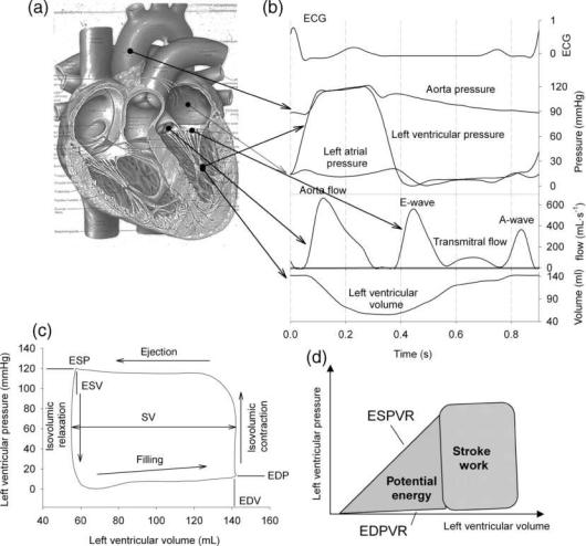
The Cardiac Cycle and Pressure–Volume Loops
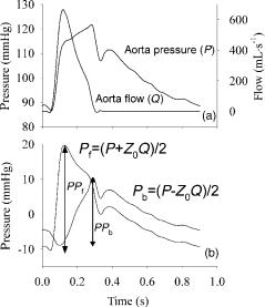
The most heavily loaded chamber is the left ventricle (LV), pumping 80 mL of blood with each contraction (70 beats min 1), with intraventricular pressure increasing from5–10 mmHg (1 mmHg ¼ 133.3 Pa) at the onset of contraction (i.e., at the end of the filling period or diastole) to 120 mmHg (6.0 kPa) in systole (ejection period) (Fig. 1). In heart physiology research, it is common to study the function of the ventricle using pressure–volume loops (PV loops; Fig. 1), with volume on the x axis and pressure on the y axis. Considering the heart at the end of diastole, it has reached its maximal volume (EDV; end-diastolic volume). Specialized pacemaker cells within the heart generate the (electrical) stimulus for the contraction, initiating the depolarization of cardiac muscle cells (myocytes). Electrical depolarization causes the muscle to contract and ventricular pressure increases. With this, the mitral valve closes, and the ventricle contracts at closed volume, with a rapidly increasing pressure (isovolumic contraction). When LV pressure becomes higher than the pressure in the aorta, the aortic valve opens, and the ventricle ejects blood. The ventricle then starts its relaxation, slowing down the ejection, with a decrease in LV pressure. At the end of ejection, the LV has reached its end-systolic volume (ESV), and LV pressure drops below the pressure in the aorta, closing the aortic valve. Relaxation then (rapidly) takes place at closed volume (isovolumic relaxation), until LV pressure drops below LA pressure and LV early filling begins (E-wave). After complete relaxation of the ventricle, contraction of the LA is responsible for an extra (late) filling wave (A-wave). The difference between EDV and ESV is the stroke volume, SV. Multiplied with heart rate, one obtains cardiac output (CO), the flow generated by the heart, commonly expressed in L min 1. The time course of cardiac and arterial pressure and flow is shown in Fig. 1.
478 HEMODYNAMICS
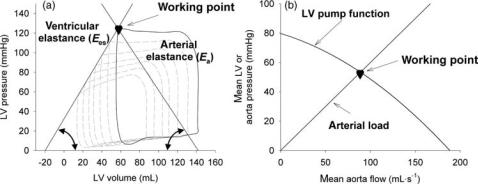
Figure 1. The heart (a), and the variation in time of pressure, flow, and volume within the left ventricle (b). Plotting left ventricular pressure as a function of volume (c), a pressure–volume loop is obtained. (d) Illustrates the association between area’s defined within the pressure–volume plane and the mechanical energy.
Time Varying Elastance and Cardiac Contractility
The intrinsic properties of cardiac muscle are responsible for making the functional pumping performance of the ventricle determined by different factors (1): the degree to which the cardiac muscle is prestretched prior to contraction (preload), the intrinsic properties of the muscle (the contractility or inotropy), the load against which the heart ejects (the afterload), and the speed with which the contraction takes place (reflected by the heart rate; chronotropy). In muscle physiology, preload is muscle length and is related to the overlap distance of the contractile proteins (actin and myosin) of the sarcomere (the basic contractile unit of a muscle cell), while afterload is the load against which a muscle strip or fiber contracts. In pump physiology, ventricular end-diastolic volume is often considered as the best approximation of preload (when unavailable, ventricular end-diastolic pressure can be used as a surrogate). To characterize afterload, one can estimate maximal ventricular wall stress (e.g., using Laplace formula), but most often, mean or systolic arterial blood pressure is taken as a measure of afterload.
Most difficult to characterize is the intrinsic contractility of the heart, which is important to know in diagnosing the severity of cardiac disease. At present, the gold standard is still considered to be the slope of the end-systolic pressure–volume relation (2,3). To fully comprehend this measure, the time varying elastance concept has to be introduced.
Throughout a cardiac cycle, cardiac muscle contracts and relaxes. The functional properties of fully relaxed muscle-at the end of diastole-can be studied in the pressure–volume plane. This relation, sometimes called the (end-) diastolic pressure–volume relation (EDPVR), is nonlinear, that is, for higher volumes, a higher increase in pressure (DP) is required to realize a given increase in volume (DV). With the volume/pressure ratio defined as compliance, the ventricle behaves less compliant (stiffer) at high volume. The EDPVR represents the passive properties of the ventricular chamber.
Similarly, if one could ‘‘freeze’’ the ventricle at its maximal contraction (as is reached at the end of systole), and measure the pressure–volume relation of the chamber in
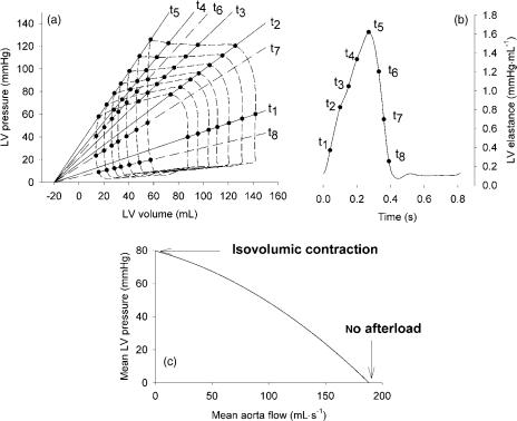
this maximally contracted state, one could assess the (end-) systolic pressure–volume relation (ESPVR) and the maximal stiffness of the ventricle. The ESPVR represents the active, contractile function of the ventricle. Throughout the cycle, the stiffness (or elastance) of the ventricle varies in between its diastolic and end-systolic value, hence the conceptual model of the time-varying elastance (Fig. 2).
The basis of this time-varying elastance model was laid by Suga et al. in the 1970s. They performed experiments in isolated hearts, and found that by increasing the initial volume of the heart (increasing preload), the maximally developed pressure in an isovolumic beat increased linearly with preload (2,3) (Frank–Starling mechanism). Obviously, the minimal pressure, determined by the passive properties, also increased. When they allowed these ventricles to eject against a quasiconstant afterload pressure, PV loops were obtained, with wider loops (higher stroke volume) being obtained for the more filled ventricles. When connecting all end-systolic points of the PV loops, it was found that the slope of this line, the endsystolic ventricular stiffness, was not different from the line obtained with the isovolumic experiments, demonstrating that it is independent of the load against which the ventricle ejects. Moreover, connecting data points on the PV loops occurring at the same instant in the cardiac cycle (isochrones), these points were also found to line up (Fig. 2). The slopes of these lines have the dimension of stiffness (DP/DV; mmHg mL 1 or Pa mL 1) or elastance (E). In addition, it is often assumed that these isochrones all have the same intercept with the volume axis (which is, however, most often not the case). This volume is called V0 and represents the volume for which the ventricle no longer develops any pressure.
HEMODYNAMICS 479
The slope of the isochronic lines, E, is given by E ¼ P/ (V V0) and can be plotted as a function of time, yielding the time varying elastance curve, E(t) (Fig. 2). The experiments of Suga and co-workers further pointed out that the maximal slope of the ESPVR, also called end-systolic (Ees) elastance, is sensitive to inotropic stimulation. The parameter Ees is, at present, still considered as the gold standard measurement of ventricular contractility.
Since these experiments, it has been shown that the ESPVR is not truly linear (4,5), especially not in conditions of high contractility or in small mammals. Since V0 is a value derived from linear extrapolation of the ESPVR, one often finds negative values, which clearly have no physiological meaning at all. Nevertheless, the time varying elastance remains an attractive concept to concisely describe ventricular function. In practice, PV loops with altered loading conditions are obtained via inflation of a balloon in one of the caval veins, reducing venous return, or with a Valsalva maneuver. The PV loops can be measured invasively with a conductance catheter (6), or by combining intraventricular pressure (measured with a catheter) with volumes measured with a medical imaging technique that is fast enough to measure instantaneous volumes during the load manipulating operations (e.g., echocardiography).
The area enclosed within the PV loop is the work performed by the heart per stroke (stroke work, SW). Furthermore, when the heart contracts, it pressurizes the volume within the ventricle, giving it a potential energy (PE). In the PV plane, PE is represented by the area enclosed within the triangle formed by V0 on the volume axis, the end-systolic point, and the left bottom corner of the PV loop (Fig. 1). The sum of SW and PE is also called the total pressure–volume area (PVA) and it has been shown
Figure 2. Pressure–volume loops recorded in the left ventricle during transient loading conditions (a), and the concept of the time-varying elastance
(b). (c) Illustrates an alternative representation of ventricular function through the pump function graph.
480 HEMODYNAMICS
that the consumption of oxygen by the myocardium, VO2, is proportional to PVA: VO2 ¼ c1PVA þ c2Ees þ c3, with c1–3 constants to be determined from experiments. The constant c1 represents the O2 cost of contraction, c2 is the O2 cost of Ca handling related to the inotropic state, and c3 is the O2 cost of basal metabolism. Mechanical efficiency can then be expressed as the ratio of SW and VO2. Recent reviews of the relation between pressure–volume area and ventricular energetics can be found in Refs. 7,8.
Another measure of ventricular function, also derived from PV loop analysis, is the so-called preload recruitable stroke work (PRSW) (9). Due to the Frank–Starling effect (10), a ventricle filled up to a higher EDV will generate a higher pressure and/or stroke volume, and hence a higher SW. Plotting SW as a function of EDV yields a quasilinear relation, of which the slope is sensitive to the contractile state of the ventricle (9).
Alternative Ways of Characterizing LV Systolic Function
Pump function of the ventricle may also be approached in a way similar to hydraulic pumps through its pump function graph (11,12), where the pressure generated by the pump (e.g., mean LV pressure) is plotted as a function of its generated flow (cardiac output). With no outflow, the ventricle contracts isovolumically, and the highest possible pressure is generated. Pumping against zero load, no pressure is built up, but outflow is maximal. The ventricle operates at some intermediate stage, in between these two extreme cases (Fig. 2). One such pump function curve is obtained by keeping heart rate, inotropy, and preload constant, while changing afterload. Although the principle is attractive, it appears to be difficult to measure pump function curves in vivo, even in experimental conditions.
Assessing Cardiac Function in Real Life
Although pressure–volume loop-based cardiac analysis still has the gold standard status in experimental work, the applicability in clinical conditions is rather limited. First, the method requires intraventricular pressure and volume. While volumes can, more and more, be measured noninvasively with magnetic resonance imaging (MRI) and even real-time three-dimensional (3D) echocardiography, the pressure requirement still implies invasive measurements. Combined pressure–volume conductance catheters are available (6), but these require calibration to convert conductance into volume data. This requires knowledge of the conductance of the cardiac structures and blood outside the cardiac chamber under study (offset correction), and an independent measurement of stroke volume for scaling of the amplitude of the conductance signal. Second, and perhaps even more important, measuring preloadrecruitable stroke work or the end-systolic pressure– volume relation requires that PV loops are recorded during transient loading conditions, which is experimentally obtained via inflation of a balloon in the caval vein to reduce the venous return and cardiac preload. It is difficult to (ethically) justify an extra puncture and the insertion of an additional catheter in patients, knowing also that these maneuvers induce secondary changes in the overall autonomic state of the patient and the release of cathechola-
mines, making this method limited to assess the pump function in a ‘‘steady state’’. To avoid the necessity of the caval vein balloon, so-called ‘‘single beat’’ methods have been proposed, where cardiac contractility is estimated from data measured at baseline steady-state conditions (13,14). The accuracy, sensitivity, and specificity of these methods, however, remains a matter of debate (15,16).
Since it is easier to measure aortic flow than ventricular volume, indicies based on the concept of ‘‘hydraulic power’’ have been proposed. As the ventricle ejects blood, it generates hydraulic power (Pwr), which is calculated as the instantaneous product of aorta pressure and flow. The peak value of power (Pwrmax) has been proposed as a measure of ventricular performance. However, due to the Frank– Starling mechanism, ventricular performance in general, and hydraulic power in particular, is highly dependent on the filling state of the ventricle, and correction of the index for EDV is mandatory. Preload-adjusted maximal power,
defined as Pwrmax/EDV2, has been proposed as a ‘‘single beat’’ (i.e., measurable during steady-state conditions)
index of ventricular performance (17). It has, however, been suggested that the factor 2 used in the denominator is not a constant, but depends on ventricular size (18). It has been demonstrated that the most correct approach is to
correct Pwrmax for (EDV V0)2, V0 being the intercept of the end-systolic pressure–volume relation (19,20). Obviously,
the index then loses its main feature, that is, the fact that it can be deduced from steady-state measurements.
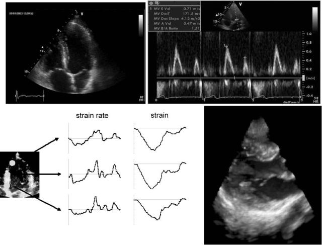
In clinical practice, cardiac function is commonly assessed with ultrasound echocardiography in its different modalities. Imaging the heart in two-dimensional (2D) planar views (2 and 4 chamber long axis views, short axis views), allows us to visually inspect ventricular wall motion and to identify noncontracting zones. With (onboard) image processing software, parameters such as ejection fraction or the velocity of circumferential fiber shortening can be derived. Echocardiography has played a major role in quantifying ‘‘diastolic function’’, that is, the filling of the heart (21,22). Traditionally, this was based on the interpretation of flow velocity patterns at the mitral valve (23) and the pulmonary veins (24). With the advent of more recent ultrasound processing tools, the arsenal has been extended. Color M-mode Doppler, where velocities are measured along a base-to-apex directed scanline, allows us to measure the propagation velocity of the mitral filling wave (25,26). More recent, much attention has been and is being paid to the velocity of the myocardial tissue (in particular the motion of the mitral annulus) (27). Further processing of tissue velocity permits us to estimate the local strain and strain rate within sample volumes positioned within the tissue. Strain and strain rate imaging are new promising tools to quantify local cardiac contractile performance (28,29). Further advances are directed toward real time 3D imaging with ultrasound and quantification of function. Some of the aforementioned ultrasound modalities are illustrated in Fig. 3.
An important domain where assessment of cardiac function is important, is in the catheterization laboratory (cathlab), where patients are ‘‘catheterized’’ to diagnose and/or treat cardiovascular disease. Access to the vasculature is gained via a large vein (the catheter then ends in the right
HEMODYNAMICS 481
Figure 3. Echocardiography of the heart. (a) Classical four-chamber view of the heart, with visualization of the four cardiac chamber; (b) transmitral flow velocity pattern; (c) strain and strain rate imaging in an apical, mid and basal segment of the left ventricle [adapted from D’hooge et al. (29)];
(d) real-time 3D visualization of the mitral valve with the GE Dimension. (Courtesy of GE Vingmed ultrasound, Horten, Norway.)
atrium/ventricle/pulmonary artery: right heart catheterization) or large artery, typically the femoral artery in the groin (the catheter then resides in the aorta/left ventricle/ left atrium: left heart catheterization). Cath-labs are equipped with X-ray scanners, allowing us to visualize cardiovascular structures in one or more planes. With injection of contrast medium, vessel structures (e.g., the coronary arteries) can be visualized (angiography) as well ventricular cavity (ventriculography). The technique, through medical image processing, allows us to estimate ventricular volumes at high temporal resolution. At the same time, arterial pressures can be monitored. Although one cannot deduce intrinsic ventricular function from pressure measurements alone, it is common to use the
peak positive (dp/dtmax) and peak negative value (dp/dtmin) of the time derivative of ventricular pressure as surrogate
markers of ventricular contractility and relaxation, respectively. These values are, however, highly dependent on ventricular preload, afterload, and heart rate, and only give a rough estimate of ventricular function. Measurement of dp/dtmax or dp/dtmin at different loading states, and
assessing the relation between changes in volume and changes in dp/dt, may compensate for the preload dependency of these parameters.
There are also clinical conditions where the physician is only interested in a global picture of cardiac function, for example, in intensive care units, where the principal question is whether the heart is able to deliver a sufficient cardiac output. In these conditions, indicator-dilution methods are still frequently applied to assess cardiac output. In this method, a known bolus of indicator substance (tracer) is injected into the venous system, and the concentration of the substance is measured on the arterial side (the dilution curve), after the blood has passed through the heart/cardiac output ¼ [amount of injected indicator]/[area under the dilution curve]. A commonly used indicator is cold saline, injected into the systemic veins, and the change in blood temperature is then measured with a catheter equipped with a thermistor, positioned in the pulmonary artery. This methodology is commonly referred to as ‘‘thermodilution’’. With valvular pathologies, as tricuspid or pulmonary valve regurgitation, the method becomes less
482 HEMODYNAMICS
accurate. The variability of the method is quite high, and the method should be repeated (three times or more) so that results can be averaged to provide a reliable estimate. Obviously, the method only yields intermittent estimates of cardiac output. Cardiac output monitors based on other measuring principles are in use, but their accuracy and/or responsiveness is still not optimal and they often require a catheter in the circulation (30,31).
Finally, it is also worth mentioning that cardiac MRI is an emerging technology, able to provide full 3D cardiac morphology and function data (e.g., with MRI tagging) (32,33). Especially for volume estimation, MRI is considered the gold standard method, but new modalities also allow us to measure intracardiac flow velocities. The high cost, the longer procedure, the fact that some materials are still banned from the scanner (e.g., metal containing pacemakers) or cause image artifacts and the limited availability of MRI scanner time in hospitals, however, make that ultrasound is still the first method of choice. For reasons of completeness, computed tomography (CT) and nuclear imaging are mentioned as medical imaging techniques that provide morphological and/or functional information on cardiac function.
The Coronary Circulation
The coronary arteries branch off the aorta immediately distal to the aortic valve (Fig. 4), and supply blood to the heart muscle itself. With their specific anatomical position, they are often considered as part of the heart, although they could as well be considered as being part of the arterial circulation. This ambiguity is also reflected in the medical specialism: coronary artery disease is the territory of the
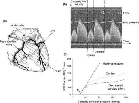
(interventional) cardiologist, and not of the angiologist. The right coronary artery mainly supplies the right heart, while the left coronary artery, which bifurcates into the left anterior descending (LAD) and left circumflex (LCX) branch, mainly supplies the left heart.
As they have to perfuse the cardiac muscle, the coronaries protrude the ventricular wall, which has a profound effect on coronary hemodynamics (34,35). Upon ventricular contraction, blood flow in the coronaries is impeded, leading to a typical biphasic flow pattern, with systolic flow impediment, and predominantly flow during the diastolic phase (Fig. 4). This pattern is most obvious in the LAD, which supplies oxygenized blood to the left ventricle. The resistance of the coronary arteries is thus not constant in time, and contains an active component. When coronary flow is plotted as a function of coronary pressure, other typical features for the coronary circulation are observed. Under normal conditions, coronary flow is highly regulated, so that blood flow is constant for a wide range of coronary perfusion pressures (35,36). The level up to which the flow is regulated is a function of the activity of the ventricle, and hence of the metabolic demands. This seems to suggest that at least two different mechanisms are involved: metabolic autoregulation (flow is determined by the metabolic demand) and myogenic autoregulation. Myogenic autoregulation is the response of a muscular vessel on an increase in pressure: the vessel contracts, reducing its diameter and increasing its wall thickness, which tends to normalize the wall stress. It is only after maximal dilatation of the coronary vessels [e.g., through infusion of vasodilating pharmacological substances such as adenosine or papaverine, or immediately following a period of oxygen deficiency (ischemia)] that autoregulation
Figure 4. (a) Anatomical situation of the coronary arteries. (b) Demonstration of flow impediment during systole. (c) Coronary flow as a function of perfusion pressure, demonstrating the aspect of autoregulation and the non-zero intercept with the pressure axis (Pzf; zero-flow pressure). (Reconstructed after Ref. 36.)
can be ‘‘switched off’’, and that the pressure-flow relation becomes linear (Fig. 4). Note, however, that the pressureflow relation does not pass through the origin: it requires a certain pressure value (zero-flow pressure Pzf) to generate any flow, an observation first reported by Bellamy et al. (37). The origin of Pzf is still not fully understood and has been attributed to (partial) vessel collapse by vascular tone and extravascular compression. This is a conceptual model, also known as the ‘‘waterfall’’ model, as flow is determined by the pressure difference between inflow and surrounding pressure (instead of outflow pressure) and pressure changes distal to the point of collapse (the waterfall) have no influence on flow (38,39). Note, however, that Pzf is often an extrapolation of pressure-flow data measured in a higher pressure range. It is plausible that the relation becomes nonlinear in the lower perfusion pressure range, due to the distensibility of the coronary vessels and compression of vessels due to intramyocardial volume shifts (35). Another model, based on the concept of an intramyocardial pump and capable of explaining phasic patterns of pressure and flow waves, was developed by Spaan et al. (35,40), and is mentioned here for reasons of completeness.
An important clinical aspect of the coronary circulation, which we will only briefly touch here, is the assessment of the severity of coronary artery stenosis (34). The stenosis forms an obstruction to flow, causes an extra pressure drop, and may result in coronary perfusion pressures too low to provide oxygen to the myocardial tissues perfused by that coronary artery. Imaging of the coronary vessels and the stenosis with angiography (in the cath-lab) is still an important tool for clinical decision making, but more and more attention has been attributed to quantification of functional severity of the stenosis. One of the most known indicies in use are the coronary flow reserve (CFR), that is, the ratio of maximal blood flow (velocity) through a coronary artery (after induction of maximal vasodilation) and baseline blood flow (velocity), with values > 2 indicating sufficient reserve and thus a subcritical stenosis. Coronary flow reserve has the drawback that flow or velocity measurements are required, which are not common in the cathlab. From that perspective, the fractional flow reserve (FFR) is more attractive, as it requires only pressure measurements. It can be shown that FFR ¼ Pd/Pa (with Pd the pressure distal to the stenosis and Pa the aorta pressure) is the ratio of actual flow through the coronary, and the hypothetical flow that would pass through the coronary in the absence of the stenosis (34,41). A FFR value >0.75 indicates nonsignificant stenosis (34). Measurement of FFR is done in conditions of maximal vasodilation, and requires ultrathin pressure catheters (pressure wires) that can pass through the stenosis without causing (too much) extra pressure drop. Other indicies combine pressure and flow velocity (42) and are, from fluid dynamic perspective, probably the best characterization of the extra resistance created by the stenosis. It deserves to be mentioned that intravascular ultrasound (IVUS) is, currently, increasingly being applied, especially when treating complex coronary lesions. In addition to quantifying stenosis severity, much research is also focused on assessing the histology of the lesions and their vulnerability and risk of rupture via IVUS or other techniques.
HEMODYNAMICS 483
THE ARTERIAL SYSTEM: DAMPING RESERVOIR AND/OR A BLOOD DISTRIBUTING NETWORK. . .
Basically, there are two ways of approaching the arterial system (43): (1) one can look at it in a ‘‘lumped’’ way, where abstraction is being made of the fact that the vasculature is a network system with properties distributed in space; or (2) one can take into account the network topology, and analyze the system in terms of pressure and flow waves propagating along the arteries in a forward and backward direction.
Irrespective of the conceptual framework within which one works, the analysis of the arterial system requires (simultaneously measured) pressure and flow, preferably measured at the upstream end of the arterial tree (i.e., immediately distal to the aortic valve). The analysis of the arterial system is largely analogous to the analysis of electrical network systems, where pressure is equivalent to voltage and flow to current. Also steming from this analogy is the fact that the arterial system is often analyzed in terms of impedance. Therefore, before continuing, the concept of impedance is introduced.
Impedance Analysis
While electrical waves are sine waves, with a zero timeaverage value, arterial pressure and flow waves are (approximately) periodical, but certainly nonsinusoidal, and their average value is different from zero (in humans, mean systemic arterial blood pressure is 100 mmHg (13.3 kPa), while mean flow is 100 mL s 1). To bypass this limitation, one can use the Fourier theorem, which states that any periodic signal, such as arterial pressure and flow, can be decomposed into a constant (the mean value of the signal) and a series of sinusoidal waves (harmonics). The frequency of the first harmonic is cardiac frequency (the fundamental frequency), while the frequency of the nth harmonic is n times the fundamental frequency.
Fourier decomposition is applicable if two conditions are fulfilled: (1) the cardiovascular system operates in steadystate conditions (constant heart rate; no respiratory effects); (2) the mechanical properties of the arterial system are sufficiently linear so that the superposition principle applies, meaning that the individual sine waves do not interact and that the sum of the effects of individual harmonics (e.g., the flow generated by a pressure harmonic) is equal to the effect caused by the original wave that is the sum of all individual harmonics.
Harmonics can be represented using a complex formalism. For the nth harmonic, the pressure (P) and flow (Q) component can be written as
Pn ¼ jPnjeiðnvtþFPn Þ Qn ¼ jQnjeiðnvtþFQn Þ
where jPnj and jQnj are the amplitudes (or modul) of the pressure and flow sine waves, having phase angles FPn and FQn (to allow for a phase lag in the harmonic), respectively. Time is indicated by t, and v is the fundamental angular frequency, given by 2p/T with T the duration of a heart cycle (RR-interval). For a heart rate of 75 beats min 1, T is 0.8 s. The fundamental frequencyis1.25Hz,andvbecomes7.85 rad s 1.
In general, 10–15 harmonics are sufficient to describe hemodynamic variables, such as pressure, flow, or volume
484 HEMODYNAMICS
(44,45). Also, to avoid aliasing, the sampling frequency should be twice as high as the frequency of the signal one is measuring (Nyquist limit). Thus, when measuring hemodynamic data in humans, the frequency response of the equipment should be > 2 15 1.25 Hz, or > 37.5 Hz. These requirements are commonly met by Hi–Fi pressure tip catheters (e.g., Millar catheters) with a measuring sensor embedded within the tip of the sensor, but not by the fluid-filled measuring systems that are frequently used in the clinical setting. Here, the measuring sensor is outside the body (directly or via extra fluid lines) connected to a catheter. Although the frequency response of the sensor itself is often adequate, the pressure signal is being distorted by the transmission via the catheter (and fluid lines and eventual connector pieces and three-way valves). The use of short, rigid, and large bore catheters is recommended, but it is advised to assess the actual frequency response of the system (as it is applied in vivo) if the pressure data is being used for purposes other than patient monitoring. Note that in small rodents like the mouse, where heart rate is as high as 600 beats min 1, the fundamental frequency is 10 Hz, posing much higher measuring equipment requirements with a frequency response flat up to 300 Hz.
Impedance Z is generally defined as the ratio of pressure and flow: Z ¼ P/Q, and thus has the dimensions of mmHg mL 1 s [kg m 4 s 1 in SI units; dyn cm 5 s in older units] if pressure is expressed in mmHg and flow in mL s 1. The parameter Z is usually calculated for each individual harmonic, and displayed as a function of frequency. Since both P and Q are complex numbers, Z is complex as well, and also has a modulus and a phase angle, except for the steady (dc) component at 0 Hz, which is nothing but the
ratio of mean pressure and mean flow (i.e., the value of vascular resistance). For all higher harmonics, the modulus of the nth harmonic is given as jZnj ¼ jPnj/jQnj, and its phase, Fz, is given as FPn FQn .
Arterial impedance requires simultaneous measurement of pressure and flow at the same location. Although it can be calculated all over the arterial tree, it is most commonly measured at the entrance of the systemic or pulmonary circulation, and is called ‘input’ impedance, often denoted as Zin. The parameter Zin fully captures the relation between pressure and flow, and is determined by all downstream factors influencing this relation (arterial network topology, branching patterns, stiffness of the vessel, vasomotor tone, . . .). In a way, it is a powerful description of the arterial circulation, since it captures all effects, but this is at the same time its greatest weakness, as it is not very sensitive to local changes in arterial system properties, such as focal atherosclerotic lesions.
The interpretation of (input) impedance is facilitated by studying the impedance of basic electrical or mechanical ‘‘building blocks’’ (43–45): (1) When a system behaves strictly resistive, there is a linear relation between the pressure (difference) and flow. Pressure and flow are always in phase, Zn is a real number and Fz is zero.
(2) In the case where there is only inertia in a system, pressure is ahead of flow; for sine waves, the phase difference between both is a quarter of a wavelength, or þ 908 in terms of phase angle. (3) In the case where the system behaves like a capacitor, flow is leading pressure, again 908 out of phase, so that Fz is 908.
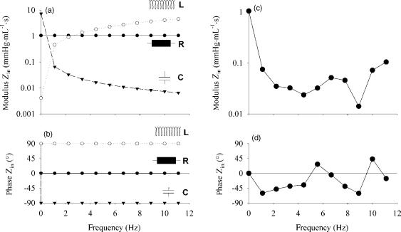
Figure 5 displays the input impedance of these fundamental building blocks, as well as Zin calculated from the
Figure 5. (a and b) Impedance modulus (a) and phase angle (b) of fundamental electrical/mechanical building blocks of the arterial system: resistance (R; 1.028 mmHg mL 1 s (137.0 106 Pa m 3 s)), inertia [L; 0.065 mmHg mL 1 s2 (8.7 106 Pa m 3 s2)] and compliance [C; 2.25 mL mmHg 1 (16.9 10 9 m3 Pa 1)]. (c and d) input impedance modulus (c) and phase (d) calculated from aortic pressure and flow given in Fig. 1.
aorta pressure and flow shown in Fig. 1. The impedance modulus drops from the value of total systemic vascular resistance at 0 Hz to much lower values at higher frequencies. The phase angle is negative up until the fourth harmonic, showing that capacitive effects dominate at these low frequencies, although the phase angle never reaches 908, indicating that inertial effects are present as well. For higher harmonics, the phase angle is close to zero, or at least oscillating around the zero value. At the same time, the modulus of Zin is nearly constant. For these high frequencies, the system seems to act as a pure resistance, and the impedance value, averaged over the higher harmonics, has been termed the characteristic impedance (Z0).
The Arterial System as a ‘‘Windkessel’’ Model
The most simple approximation of the arterial system is based on observations of reverend Stephen Hales (1733), who drew the parallel between the heart ejecting in the arterial tree, and the working principle of a fire hose (46). The pulsatile action of the pump is damped and transformed into a quasicontinuous outflow at the downstream
HEMODYNAMICS 485
end of the system, that is, the outflow nozzle for the fire hose and the capillaries for the cardiovascular system. In mechanical terms, this type of system behavior can be simulated with two mechanical components: a buffer reservoir (compliant system) and a downstream resistance. In 1899, Otto Frank translated this into a mathematical formulation (47,48), and it was Frank who introduced the terminology ‘‘windkessel models’’, windkessel being the German word for air chamber, as the buffer chamber used in the historical fire hose. The windkessel models are often described as their electrical analogue (Fig. 6).
The Two-Element Windkessel Model. While there are many different ‘‘windkessel’’ models in use (49,50), the two basic components contained within each model are a compliance element, C (mL mmHg 1 or m3 Pa 1), and a resistor element, R (mmHg mL 1 s or Pa m 3 s in SI units). The compliance element represents the volume change associated with a unit change in pressure; R is the pressure drop over the resistor associated with a unit flow. In diastole, when there is no new inflow of blood into the compliance, the arterial pressure decays exponentially following P(t) ¼ P0e t/RC. The parameter RC is the product
Figure 6. (a and b) Electrical analog and mechanical representation of a twoand three-element windkessel model. (c) Agreement between measured pressure, and the pressure obtained after fitting a twoand three-element windkessel model to the pressure (1 mmHg ¼ 133.3 Pa) and flow data from Fig. 1. Model parameters are R ¼ 1.056 mmHg mL 1 s (140.8 106 Pa m 3 s) and C ¼ 2.13 mL mmHg 1 (16.0 10 9 m3 Pa 1) for the two-element windkessel model; R ¼ 1.028 mm
Hg mL 1 s (137.0 106 Pa m 3 s). C ¼ 2.25 mL mmHg 1 (16.9 10 9 m3 Pa 1) and Z0 ¼ 0.028 mmHg mL 1 s (3.7 106 Pa m 3 s) for the three-element windkessel model. (d and e) Input impedance
modulus (d) and phase angle (e) of these lumped parameter models and their match to the in vivo measured input impedance (1 mmHg mL 1 s ¼ 133.3 106 Pa m 3 s).

486 HEMODYNAMICS
of R and C and is called the arterial decay time. The higher the RC time, the slower the pressure decay. It is the time required to reduce P0 to 37% of its initial value (note that the 37% is a theoretical value, usually not reached in vivo because the next beat impedes a full pressure decay). One can make use of this property to estimate the arterial compliance: By fitting an exponential curve to the diastolic decaying pressure, RC is obtained and thus, when R is known we also know C (49,51–53). This method is known as the decay time method.
For typical hemodynamic conditions in humans at rest (70 beats min 1, systolic/diastolic, and mean pressure of 120 (16.0 kPa), 80 (10.7 kPa), and 93 (12.4 kPa) mmHg
respectively, stroke volume 80 mL), mean flow is 93 mL s 1 (0.93 10 4 m3 s 1), and R is 1 mmHg (mL s 1)
(133.3 106 Pa m 3 s). Assuming that the whole stroke volume is buffered in systole, C can be estimated as the ratio of stroke volume and pulse pressure (systolic–diasto- lic pressure difference), 2 mL mmHg 1 (1.50 10 8 m3 Pa 1). This value is considered as an overestimation of the actual arterial compliance (49,54). In humans, RC time is thus of the order of 1.5–2 s.
The question, How well does a windkessel model represents the actual arterial system?, can be answered by studying the input impedance of both. In complex formulation, the input impedance of a two-element windkessel model is given as
R
Zi WK2 ¼ 1 þ ivRC
with i the complex constant, and v ¼ 2pf, f is the frequency. The dc value (0 Hz) of Zin is thus R; at high frequencies, it becomes zero. The phase angle is 0 at 0 Hz, and 908 for all other frequencies. Compared to input impedance as measured in mammals, the behavior of a two-element windkessel model reasonably represents the behavior of the arterial system for the low frequencies (up to third harmonic), but not for higher frequencies (43,49,54) (Fig. 6). This means that it is justified to use the model for predicting the low frequency behavior of the arterial system, that is, the low frequency response to a flow input. This property is used in the so-called ‘‘pulse pressure method’’, an iterative method to estimate arterial compliance: with R assumed known, the pulse pressure response of the two-element windkessel model to a (measured) flow stimulus is calculated with varying values of C. The value of C yielding the pulse pressure response matching the one measured in vivo, is considered to be the correct one (55). Compared to the decay time method, the advantage is that the pulse pressure method is insensitive to deviations of the decaying pressure from the true exponential decay (53).
The Three-Element and Higher Order Windkessel Models. The major shortcoming of the two-element windkessel model is the inadequate high frequency behavior (43,49,56). Westerhof et al.resolved this problem by adding a third resistive element proximal to the windkessel, accounting for the resistive-like behavior of the arterial system in the high frequency range (56). The third element represents the characteristic impedance of the proximal
part of the ascending aorta, and integrates the effects of inertia and compliance. Adding the element, the input impedance of the three-element windkessel model becomes
R
Zi WK3 ¼ Z0 þ 1 þ ivRC
it making the phase angle negative for lower harmonics, but returns to zero for higher harmonics, where the impedance modulus asymptotically reaches the value of Z0. For the systemic circulation, the ratio of Z0 and R is 0.05–0.1 (57).
The major disadvantage of the three-element windkessel model is the fact that Z0, which should represent the high frequency behavior of the arterial system, plays a role at all frequencies, including at 0 Hz. This has the effect that, when the three-element windkessel model is used to fit data measured in the arterial system, the compliance is systematically overestimated (53,58): the only way to ‘‘neutralize’’ the contribution of Z0 at the low frequencies, is to artificially increase the compliance of the model. The ‘‘ideal’’ model would incorporate both the low frequency behavior of the two-element windkessel model, and the high frequency Z0, though without interference of the latter at all frequencies. This can be achieved by adding an inertial element in parallel to the characteristic impedance, as demonstrated by Stergiopulos et al. (59), elaborating on a model first introduced by Burattini et al. (60). For the DC component and low frequencies, Z0 is bypassed through the inertial element. For the high frequencies, Z0 takes over. It has been demonstrated, fitting the fourelement windkessel model to data generated using an extended arterial network model, that L effectively represents the total inertia present in the model (59).
Obviously, by adding more elements, it is possible to develop models that are able to further enhance the matching between model and arterial system behavior (49,50), but the uniqueness of the model may not be guaranteed, and the physiological interpretation of the model elements is not always clear.
Although lumped parameter models cannot explain all aspects of hemodynamics, they are very useful as a concise representation of the arterial system. Mechanical versions are frequently used in hydraulic bench experiments, or as highly controllable afterload systems for in vivo experiments. An important field of application of the mathematical version is for parameter identification purposes: fitting arterial pressure and flow data measured in vivo to these models, the arterial system can be characterized and quantified (e.g., the total arterial compliance) through the model parameter values (43,49).
It is important to stress that these lumped models represent the behavior of the arterial system as a whole, and that there is no relation between model components and anatomical parts of the arterial tree (43). For example, although Z0 represents the properties of the proximal aorta, there is no drop in mean pressure along the aorta, which one would expect if the three-element windkessel model were to be interpreted in a strict anatomical way. The combination of elements simply yields a model that represents the behavior of the arterial system as it is seen by the heart.

HEMODYNAMICS 487
Figure 7. (a) Shows both pressure (1 mmHg ¼ 133.3 Pa) and flow velocity measured along the arterial tree in a dog [after Ref. (44).] (b) Pressure wave forms measured between the aortic valve (AoV) and the terminal aorta (Term Ao) in one patient. [Modified from Ref. 61.]
Wave Propagation and Reflection in the Arterial Tree
As already stressed, lumped parameter models simply represent the behavior of the arterial system as a whole, and as seen by the heart. As soon as the model is subjected to flow or pressure, there is an instantaneous effect throughout the whole model. This is not the case in the arterial tree: when measuring pressure along the aorta, it can be observed that there is a finite time delay between the onset of pressure rise and flow in the ascending and distal aorta (Fig. 7). The pressure pulse travels with a given speed from the heart toward the periphery.
When carefully analyzing pressure wave profiles measured along the aorta, several observations can be made: (1) there is a gradual increase in the steepness of the wave front; (2) there is an increase in peak systolic pressure (at least in the large-to-middle sized arteries); (3) diastolic blood pressure is nearly constant, and the drop in mean blood pressure (due to viscous losses) is negligible in the large arteries. The flow (or velocity) wave profiles exhibit the same time delay in between measuring locations, but their amplitude decreases. Also, by comparing the pressure and flow wave morphology, one can observe that these are fundamentally different.
In the absence of wave reflection (assuming the aorta to be a uniform, infinitely long elastic tube), dissipation would only lead to less steep wave fronts, and damping of maximal pressure. Also, in these conditions, one would expect similarity of pressure and flow wave morphology. Thus, the above observations can only be explained by wave reflection. This is, of course, not surprising given the complex anatomical structure of the arterial tree, with geometric and elastic tapering (the further away from the heart, the stiffer the vessel), its numerous bifurcations, and the arterioles and capillaries making the distal terminations.
The Arterial Tree as a Tube. Despite the complexity described above, arterial wave reflection is often approached in a simple way, conceptually considering the arterial tree
as a single tube [or T-tube (62)], with one (or 2) discrete reflection site(s) at some distance from the heart. Within the single tube concept, the arterial tree is seen as a uniform or tapered (visco-)elastic tube (63,64), with an ‘‘effective length’’ (65,66), and a single distal reflection site. The input impedance of such a system can be calculated, as demonstrated in Fig. 8 for a uniform tube of length 50 cm, diameter 1.5 cm, Z0 of 0.275 mmHg mL 1 s (36.7 106 Pa m 3 s) and wave propagation speed of 6.2 m s 1. The tube is ended
Figure 8. Input impedance modulus and phase of a uniform tube with length 50 cm, diameter 1.5 cm, characteristic impedance of 0.275 mmHg mL 1 s (36.7 106 Pa m 3 s) and wave propagation speed of 6.2 m s 1. The tube is ended by a (linear) resistance of 1 mmHg mL 1 s (133.3 106 Pa m 3 s).
488 HEMODYNAMICS
by a (linear) resistance of 1 mmHg mL 1 s (133.3 106 Pa m 3 s). The impedance mismatch between the tube and its terminal resistance gives rise to wave reflections and oscillations in the input impedance pattern, and many features, observed in vivo (67), can be explained on the basis of this model.
Assume there is a sinusoidal wave running in the system with a wavelength l being four times the length of the tube. This means that the phase angle of the reflected wave, when arriving back at the entrance at the tube, will be 1808 out of phase with respect to the forward wave. The sum of the incident and reflected wave will be zero, since they interfere in a maximally destructive way. If this wave is a pressure wave, measured pressure at the entrance of the tube will be minimal for waves with this particular wave length. There is a relation between pulse wave velocity (PWV), l, and frequency f (i.e., l ¼ PWV/f). Thus, in an input impedance spectrum, the frequency fmin, where input impedance is minimal, corresponds to a wave with a wavelength that is equal to four times the distance to the
reflection site, L,: 4L ¼ PWV/fmin, or L ¼ PWV/4fmin and fmin ¼ PWV/4L. Applied to the example of the tube, fmin is expected at 6.2/2 ¼ 3.1 Hz. This equation is known as the
‘‘quarter wavelength’’ formula, and is used to estimate the effective length of the arterial system.
Although the wave reflection pattern in the arterial system is complex (68), pressure (P) and flow (Q) are mostly considered to be composed of only one forward running component, Pf (Qf) and one backward running component, Pb (Qb), where the single forward and backward running components are the resultant of all forward and backward traveling waves, including the forward waves that result from rereflection at the aortic valve of backward running waves (69).
At all times,
P ¼ Pf þ Pb and Q ¼ Qf þ Qb
Furthermore, if the arterial tree is considered as a tube, defined by its characteristic impedance Z0, the following relations also apply:
Z0 ¼ Pf =Qf ¼ Pb=Qb
since Z0 is the ratio of pressure and flow in the absence of wave reflection (43–45), which is the case when only forward or backward running components are taken into consideration. The negative sign in the equation above appears because the flow is directional, considered positive in the direction away from the heart, and negative toward the heart, while the value of the pressure is insensitive to direction.
Combining these equations, P ¼ Pf Z0Qb ¼ Pf Z0 (Q Qf) ¼ 2Pf Z0Q, so that
Pf ¼ ðP þ Z0QÞ=2
Similarly, it can be deduced that
Pb ¼ ðP Z0QÞ=2
These equations were first derived by Westerhof et al., and are known as the linear wave separation equations (67). In principle, the separation should be calculated on individual
Figure 9. Application of linear wave separation analysis to the pressure (1 mmHg ¼ 133.3 Pa) and flow data of Fig. 1. The ratio of PPb and PPf can be used as a measure of wave reflection magnitude.
harmonics, and the net Pf and Pb wave then follows from summation of all forward and backward harmonics. In practice, however, the equations are often used in the time domain, using measured pressure and flow as input. Note, however, that wave reflection only applies to the pulsatile part of pressure and flow, and mean pressure and flow should be subtracted from measured pressure and flow before applying the equations. An example of wave separation is given in Fig. 9.
Note also that wave separation requires knowledge of characteristic impedance, which can be estimated both in the frequency and time domain (70). When discussing input impedance, it was already noted that for the higher harmonics (> fifth harmonic), Zin fluctuates around a constant value, Z0, and with a phase angle approaching zero. Assuming wave speed to be 5 m s 1, the wave length l for these higher harmonics (e.g., the fifth harmonic for a heart rate of 60 beats min 1), being the product of the wave speed and wave period (0.2 s) becomes shorter (1 m) than the average arterial pathlength. Waves reflect at distant locations throughout the arterial tree (with distal ends of vascular beds < 50 cm to 2 m away from the heart in humans), return back to the heart with different phase angles and destructively interfere with each other, so that the net effect of the reflected waves appears inexistent. For these higher harmonics, the arterial system thus appears reflectionless, and under these conditions, the ratio of pressure and flow is, by definition, the characteristic impedance. Therefore, averaging the input impedance modulus of the higher harmonics, where the phase angle is about zero, yields an estimate of the characteristic impedance (43–45).
Characteristic impedance can also be estimated in the time domain. In early systole, the reflected waves did not yet reach the ascending aorta, and in the early systolic ejection period, the relation between pressure and flow is
HEMODYNAMICS 489
linear, as can be observed when plotting P as a function of Q (70,71). The slope of the Q–P relationship during early systole is the time domain estimate of Z0, and is in good agreement with the frequency domain estimate (70).
Both the time and frequency domain approach, however, are sensitive to subjective criteria, such as the selection of the early systolic ejection period, or the selection of the harmonic range that is used for averaging.
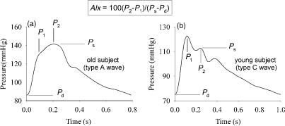
Pathophysiological Consequences of Arterial Wave Reflection. Figure 10 displays representative carotid artery pressure waves ( aorta pressure) for a young subject, (b), and for an older, healthy subject, (a). It is directly observed that the morphology of the pressure wave is fundamentally different. In the young subject, pressure first reaches its maximal systolic pressure, and an ‘‘inflection point’’ is visible in late systole, generating a late shoulder (P2). In the older subject, this inflection point appears in early systole, generating an early shoulder (P1).
Measurements of pressure along different locations in the aorta, conducted by Latham et al. (67), showed that, when the foot of the wave on one hand, and the inflection point on the other, are interconnected (Fig. 7): (1) these points seem to be aligned on two lines; (2) the lines connecting these characteristic marks intersect. This pattern is consistent with the concept of a pressure wave being generated by the heart, traveling down the aorta, reflect, and superimpose on the forward going wave. The inflection point is then a visual landmark, designating the moment in time where the backward wave becomes dominant over the forward wave (61).
In young subjects, the arteries are most elastic (deformable), and pulse wave velocity (see below) is much lower than in older subjects, or in patients with hypertension or diabetes. In the young, it takes more time for the forward wave to travel to the reflection site, and for the reflected wave to arrive at the ascending aorta. Both interact only in late systole (late systolic inflection point), causing little extra load on the heart. In older subjects, on the other hand, PWV is much higher, and the inflection point shifts to early systole. The early arrival of the reflected wave literally boosts systolic pressure, causing pressure augmentation, and augmenting the load on the heart (72). At the same time, the early return of the reflected wave impedes ventricular ejection, and thus may have a negative impact on stroke volume (72,73). An increased load on the heart increases the energetic cost to maintain stroke
Figure 10. Typical pressure wave contours measured noninvasively at the common carotid artery with applanation tonometry in a young and old subject, and definition of the ‘‘augmentation index’’ (AIx) (1 mmHg ¼ 133.3 Pa). See text for details.
volume, and will initiate cardiac compensatory mechanisms (remodeling), which may progress into cardiac pathology (74–76).
Wave Intensity Analysis. With its origin in electrical network theory, much of the arterial function analysis, including wave reflection, is done in the frequency domain. Besides the fact that this analysis is, strictly speaking, only applicable in linear systems with periodic signal changes, the analysis is quite complex due to the necessity of Fourier decomposition, and it is not intuitively comprehensible. An alternative method of analysis, performed in the time domain and not requiring linearity and periodicity is the analysis of the wave intensity, elaborated by Parker and Jones in the late 1980s (77).
Disturbances to the flow lead to changes in pressure (dP) and flow velocity (dU), ‘‘wavelets’’, which propagate along the vessels with a wave speed (PWV), as defined above. By accounting for conservation of mass and momentum, it can be shown that
dP ¼ PWVrdU
where the ‘‘þ’’ denotes a forward traveling wave (for a defined positive direction), while ‘‘ ’’ denotes a backward traveling wave. This equation is also known as the waterhammer equation. Waves characterized by a dP > 0, that is, a rise in pressure, are called compression waves, while waves with dP < 0 are expansion waves. Note that this terminology still reflects the origin of the theory in gas dynamics.
Basically, considering a tube, with left-to-right as the positive direction, there are four possible types of waves: (1) Blowing on the left side of the tube, pressure rises (dP > 0), and velocity increases (dU > 0). This is a forward compression wave. (2) Blowing on the right side of the tube, pressure increases (dP > 0), but velocity decreases (dU < 0) with our convention. This is a backward compression wave. (3) Sucking on the left side of the tube, pressure decreases (dP < 0), as well as the velocity (dU < 0), but the wavefront propagates from left to right. This wave type is a forward expansion wave. (4) Finally, one can also suck on the right side of the tube, causing a decrease in pressure (dP < 0) but an increase in velocity (dU > 0). This is a backward expansion wave.
The nature of a wave is most easily comprehended by analysing the wave intensity, dI, which is defined as the product of dU and dP, and is the energy flux carried by the
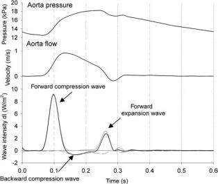
490 HEMODYNAMICS
Figure 11. The concept of wave intensity analysis, applied to pressure and flow measured in the ascending aorta of a dog.
wavelet. It can be deduced from the above that dI is always positive for forward running waves, and always negative for a backward wave. When dI is positive, forward waves are dominant; otherwise, backward waves are dominating. Analysis of dP reveals whether the wave is a compression or an expansion wave. Figure 11 shows the wave intensity calculated from pressure and flow velocity measured in the ascending aorta of a dog (71). A typical wave intensity pattern is characterized by three major peaks. The first one is a forward compression wave, associated with the ejection of blood from the ventricle. The second positive peak is associated with a forward running wave, but dP < 0, and this second peak is thus a forward running expansion wave, due to ventricular relaxation, slowing down the ejection from the heart. During systole, reflected waves are dominant, resulting in a negative wave intensity, but with, in this case, positive dP. The negative peak is thus a backward compression wave, resulting from the peripheral wave reflections.
Further, note that similar to Westerhof’s work (69), the wavelets dP and dU also can be decomposed in the forward and backward components (71). It can be derived that
dP ¼ |
1 |
ðdP rPWV dUÞ |
and dU ¼ |
1 |
|
dP |
dU |
|
|
|
|||||
2 |
2 |
rPWV |
The total forward and backward pressure and flow wave can be obtained as
Xt
Pþ ¼ Pd þ dPþ
t¼0
with Pd the diastolic blood pressure, which is added to the
forward wave, and P ¼ Pt dP (71). Similarly, for the
t¼0
forward and backward velocity wave, it applies that
X |
X |
t |
t |
Uþ ¼ |
dUþ and U ¼ dU |
t¼0 |
t¼0 |
Wave Intensity in itself, dI, can also be separated in a net forward and backward wave intensity: dIþ ¼ dPþdUþ and dI ¼ dP dU with dI ¼ dIþ þ dI .
Wave intensity is certainly an appealing method to gain insight into complex wave (reflection) patterns, as in the arterial system, and the use of the method is growing (78– 80). The drawback of the method is the fact that dI is calculated as the product of two derivatives dP and dU, and thus is highly sensitive to noise in the signal. Adequate filtering of basic signals and derivatives is mandatory. As for the more ‘‘classic’’ impedance analysis, it is also required that pressure and flow be measured at the exact same location, and preferably at the same time.
Assessing Arterial Hemodynamics in Real Life
Analyzing Wave Propagation and Reflection. The easiest approach of analyzing wave reflection is to simply quantify the global effect of wave reflection on the pressure wave morphology. This can be done by formally quantifying the observation of Murgo et al. (61), and is now commonly known as the augmentation index (AIx). This index was first defined in the late 1980s by Kelly et al. (81). Although different formulations are used, AIx is nowadays most commonly defined as the ratio of the difference between the ‘‘secondary’’ and ‘‘primary peak’’, and pulse pressure: AIx ¼ 100 (P2 P1)/(Ps Pd), and expressed as a percentage (Fig. 10). For A-type waves (Fig. 10) with a shoulder preceding systolic pressure, P1 is a pressure value characteristic for the shoulder, while P2 is systolic pressure. These values are positive. For C-type waves, the shoulder follows systolic pressure, and P1 is systolic pressure, while P2 is a pressure value characteristic for the shoulder, thus yielding negative values for AIx (Fig. 10). There are also alternative formulations in use, for example, 100(P2 Pd)/ (P1 Pd), which always yields a positive value (< 100% for C-type waves, and > 100% for A-type waves). Both are, of course, mathematically related to each other. Since AIx is an index based on pressure differences and ratios, it can be calculated from noncalibrated pressure waveforms, which can be obtained noninvasively using techniques such as applanation tonometry (see below). In the past 5 years, numerous studies have been published using AIx as a quantification of the contribution of wave reflection to arterial load.
It is, however, important to stress that AIx is an integrated measure and that its value depends on all factors influencing the magnitude and timing of the reflected wave: pulse wave velocity, magnitude of wave reflection, and the distance to the reflection site. This AIx is thus strongly dependent on body size (82). In women, the earlier return of the reflected wave leads to higher AIx. The relative timing of arrival of the reflected wave is also important, so that AIx is also dependent on heart rate (83). For higher heart rates, systolic ejection time shortens, so that the reflected wave arrives relatively later in the cycle, leading to an inverse relation between heart rate and AIx.
Instead of studying the net effect of wave reflection, one can also measure pressure and flow (at the same location) and separate the forward and backward wave using the
aforementioned formulas. An example is given in Fig. 9, using aorta pressure and flow from Fig. 1. The ratio of the amplitude of Pb (PPb) and Pf (PPf) then yields an easy measure of wave reflection, which can be considered as a wave reflection coefficient, although it is to be emphasized that it is not a reflection coefficient in a strict sense. It is not the reflection coefficient at the site of reflection, but at the upstream end of the arterial tree and thus also incorporates the effects of wave dissipation, playing a role along the pathlength for the forward and backward component.
Another important determinant of the augmentation index is pulse wave velocity, which is an interesting measure of arterial stiffness in itself. This is easily demon-
strated via the theoretical Moens–Korteweg equation for a |
|
Young elasticity modulus (400–1200 |
p |
uniform 1D tube, stating that PWV |
¼ Eh=rD with E the |
|
kPa for arteries), r the |
density of blood ( 1060 kg m 3), h the wall thickness, and D the diameter of the vessel. Another formula, sometimes
used, is the so-called Bramwell–Hill (84) equation: PWV ¼ |
||
p |
|
pA the area compliance, @A/@P. For |
|
A@P=r@A ¼ |
A=r 1= CA with P intra-arterial pressure, A |
cross-sectional area and C
unaltered vessel dimensions, an increase in stiffness (increase in E, decrease in CA) yields an increase in PWV. The most common technique to estimate PWV is to measure the time delay between the passage of the pressure, flow, or diameter distension pulse at two distinct locations, for example, between the ascending aorta (or carotid artery) and the femoral artery (85). These signals can be measured noninvasively, for example, with tonometry (86,87) (pressure pulse) or ultrasound [flow velocity, vessel diameter distension (88,89)]. Reference work was done by Avolio et al., who measured PWV is large cohorts in Chinese urban and rural communities (90,91).
When the input impedance is known, which implies that pressure and flow are known, the ‘‘effective length’’ of the arterial system, that is, the distance between the location
HEMODYNAMICS 491
where the input impedance is measured and an ‘‘apparent’’ reflection site at a distance L, can be estimated using the earlier mentioned quarter wavelength formula. Murgo et al. found the effective length to be 44 cm in humans (61), which would suggest a reflection site near the diaphragm, in the vicinity of where the renal arteries branch off the abdominal aorta. Latham et al. demonstrated that local reflection is higher at this site (67), but one should keep in mind that the quarter wavelength formula is based on a conceptual model of the arterial system, and the apparent length does not correspond to a physical obstruction causing the reflection. Nevertheless, there is still no clear picture of the major reflection sites, which is complex due to the continuous branching, the dispersed distal reflection sites, and the continuous reflection caused by the geometric and elastic tapering of the vessels (45,64,67,68,92–96).
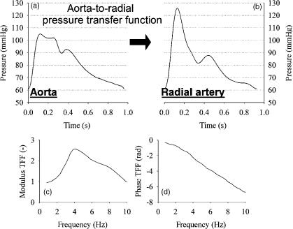
Central and Peripheral Blood Pressure: On the Use of Transfer Functions. Wave travel and reflection generally result in an amplification of the pressure pulse from the aorta (central) toward the periphery (brachial, radial, femoral artery) (44,45). Since clinicians usually measure blood pressure at the brachial artery (cuff sphygmomanometry), this implies that the pressure measured at this location is an overestimation of central pressure (97,98). It is the latter against which the heart ejects in systole, and which is therefore of primary interest.
In the past few years, much attention has been attributed to the relation between radial artery and central pressure (99–102). The reason for this is that radial artery pressure pulse is measurable with applanation tonometry, a noninvasive method (86,87,103). The relation between central and radial artery pressure can be expressed with a ‘‘transfer function’’, most commonly displayed in the frequency domain (Fig. 12). The transfer function expresses
Figure 12. Demonstration of the aorta-to-radial pressure pulse amplification: (a and b) are carotid (as substitute for aorta pressure) and radial artery pressure measured in the same subject with applanation tonometry (1 mmHg ¼ 133.3 Pa). (c and d) Display the modulus and phase angle of the radial-to-aorta transfer function as published by Ref. (99).
492 HEMODYNAMICS
the relation between the individual harmonics at both locations, with a modulus (damping or amplification of the harmonic) and a phase angle (the time delay). In humans, the aorta-to-radial transfer function shows a peak4 Hz, so that amplification is maximal for a harmonic of that frequency (99,101). It has been demonstrated that the transfer function is surprisingly constant, with albeit little variation among individuals (99). It is this observation that led to the use of generalized transfer functions, embedded in commercial systems, that allow us to calculate central pressure from a peripheral pressure measurement (104). In these systems, the transfer is commonly done using a time domain approach [autoregressive exogenous (ARX) models (100)]. There have been attempts to ‘‘individualize’’ the transfer function, but until now these attempts were unsuccessful (105). The general consensus appears to be that the generalized transfer function can be used to estimate central systolic blood pressure and pulse pressure (104), but that one should be cautious when using synthesized central pressures for assessing parameters based on details in the pressure wave (e.g., the augmentation index) (106). The latter requires high frequency information that is more difficult to guarantee with a synthesized curve, both due to the increase in scatter in the generalized transfer function for higher frequencies, and the absence of high frequency information in the peripherally measured pressure pulse (99,107).
One more issue worth noting is the fact that the radial- to-aorta transfer function peaks at 4 Hz (in humans), which implies that the peripheral pulse amplification is frequency, and thus heart rate dependent (83,108,109). In a pressure signal, most power is embedded within the first two to three harmonics. When heart rate shifts from 60 to 120 beats/min (e.g., during exercise), the highest amplification thus occurs for these most powerful, predominant harmonics, leading to a more excessive pressure amplification. This means, conversely, that the overestimation of central pressure by a peripheral pressure measurement is a function of heart rate. As such, the effect of drugs that alter the heart rate (e.g., beta blockers, slowing down heart rate) may not be fully reflected by the traditional brachial sphygmomanometer pressure measurement (97,98).
Practical Considerations. The major difficulty, transferring experimental results into clinical practice, is the accurate measurement of the data necessary for the hemodynamic analysis. Nevertheless, there are noninvasive tools available that do permit ‘‘full’’ noninvasive hemodynamic assessment in clinical conditions, as possible with central pressure and flow.
Flow is at present rather easy to measure with ultrasound, using pulsed Doppler modalities. Flow velocities can be measured in the left ventricular outflow tract and, when multiplied with outflow tract cross-section, be converted into flow. Also, velocity-encoded MRI can provide aortic blood flow velocities.
As for measuring pressure, applanation tonometry is an appealing technique, since it allows us to measure pressure pulse tracings at superficial arteries such as the radial, brachial, femoral, and carotid artery (86,87,103,110,111). The carotid artery is located close to the heart, and is often
used as a surrogate for the ascending aorta pulse contour (87,111). Others advocate the use of a transfer function to obtain central pressure from radial artery pressure measurement (104), but generalized transfer functions do not fully capture all details of a central pressure (106). Nevertheless, applanation tonometry only yields the morphology of the pressure wave and not absolute pressure values (although this is theoretically possible, but virtually impossible to achieve in practice). For the calibration of the tracings, one still relies on brachial cuff sphygmomanometry (yielding systolic and diastolic brachial blood pressure). Van Bortel et al. validated a calibration scheme in which first a brachial pressure waveform is calibrated with sphygmomanometer systolic and diastolic blood pressure (81,112). Averaging of this calibrated curve subsequently yields mean arterial blood pressure. Pulse waveforms at other peripheral locations are then calibrated using diastolic and mean blood pressure. Alternatively, one can use an oscillometric method to obtain mean arterial blood pressure, or estimate mean arterial blood pressure from systolic and diastolic blood pressure using the two-third/ one-third rule of thumb (mean blood pressure ¼ 23 diastolic þ 13 systolic pressure). With the oscillometric method, one makes use of the oscillations that can be measured within the cuff (and in the brachial artery) when the cuff pressure is lowered from a value above systolic pressure (full occlusion) to a value below diastolic pressure (no occlusion).
Nowadays, ultrasound vessel wall tracking techniques also allow us to measure the distension of the vessel upon the passage of the waveform (88,113). These waveforms are quasiidentical to the pressure waveforms [but not entirely, since the pressure–diameter relationship of blood vessels is not linear (114,115)] and can potentially be used as an alternative for tonometric waveforms (112,116).
When central pressure and flow are available, the arterial system can be characterized using all described techniques, from impedance analysis, parameter estimation by means of a lumped parameter windkessel or tube model, analysis of wave reflection, and so on. The augmentation index can be derived from pressure data alone. A parameter that is certainly relevant to measure in addition to pressure and flow is pulse wave velocity, as it provides both functional information, and helps to elucidate wave reflection. For measuring the transit time (e.g., from carotid to femoral) of the arterial pressure pulse, the flow velocity wave or the diameter distension wave is the most commonly applied technique (85).
HEART–ARTERIAL COUPLING
The main function of the heart is to maintain the circulation, that is, to provide a sufficient amount of blood at sufficiently high pressures to guarantee the perfusion of vital organs, including the heart itself. Arterial pressure and flow arise from the interaction between the ventricle and the arterial load. In the past few years, the coupling of the heart and the arterial system in cardiovascular pathophysiology has been recognized (74–76,117,118). With ageing or in hypertension, for example, arterial stiffening leads to an increase of the pressure pulse and an early
HEMODYNAMICS 493
return of reflected waves, increasing the load on the heart (73,119), which will react through adaptation (remodeling) to cope with the increased afterload.
Factors affecting ventricular pump function are preload (venous filling pressure and/or end diastolic volume EDV), heart rate, and the intrinsic contractile function of the heart muscle (here assumed to be best represented by the slope of the end-systolic PV relation, Ees). The two main mechanical afterload parameters determining systolic and pulse pressure are total peripheral resistance (R) and total arterial compliance (C) (120,121). Arterial blood pressure and flow are thus determined by a limited number of cardiac and arterial mechanical factors.
The most common framework, however, to study the heart–arterial (or ventricular–vascular) coupling, is the Ea Ees framework (23,122–124), where Ea is effective arterial elastance (125), and where Ea/Ees is a parameter reflecting heart–arterial coupling. In the pressure–volume plane, Ea is the slope of the line connecting the end-systolic point (ESV, ESP) with the end-diastolic volume point on the volume axis (EDV, 0) (Fig. 13). As such, Ea ¼ ESP/SV, with SV the stroke volume. The parameter Ea can be written as a function of three-element windkessel parameters describing the arterial system (125), but it has been shown that Ea can be approximated as R/T with T the duration of the cardiovc cycle (124,126).
The first major advantage of this framework is that it allows us to graphically study the interaction between the heart and the arterial system. Cardiac function is characterized by the ESPVR, which is a fully defined line in the PV plane. For a given preload (EDV) and arterial stiffness Ea, the line characterizing the arterial system can be drawn as well. The intersection of these two lines determines the end-systolic point (ESV, ESP), and thus the stroke volume and (end-)systolic pressure (Fig. 13).
Second, the analysis in the PV plane also allows us to calculate some energetic parameters, and to relate them to Ea/Ees. It can be shown that SW is maximal only when
Ea ¼ Ees. Thus when Ea/Ees ¼ 1. Mechanical efficiency is maximal when Ea/Ees ¼ 0.5, when arterial elastance is one-
half of the end-systolic elastance (124). In normal hearts, the heart operates in conditions with an Ea/Ees ratio in the range 0.5:1, and it has been shown that this ratio is preserved in normal aging (74,75). Arterial stiffening is thus paralleled by an increase in ventricular end-systolic stiffness. This happens even in patients with heart failure,
Figure 13. Heart–arterial coupling using the Ea–Ees (a) of the pump function graph (b) framework. In both cases, the intersection between the curves characterizing the ventricle and the arterial system determines the working point of the cardiovascular system.
but with preserved ejection fraction (76). In this patient population, both Ea and Ees are higher than expected with normal ageing, but the ratio is more or less preserved.
Although the Ea/Ees parameter certainly has its value, it has been shown under experimental conditions that the Ea/ Ees range, where the heart operates near optimal efficiency, is quite broad (122,127). Thus the parameter is not a very sensitive tool to detect ‘‘uncoupling’’ of the heart and the arterial system, which commonly implies a increase in Ea and a poorer ventricular function (depressed Ees) leading to increased Ea/Ees ratios (128,129). Also, one should not focus only on the coupling, but also on the absolute values of Ea and Ees. Increased stiffening leads to hypertensive response in exercise, where small changes in volume (filling volumes, stroke volumes) have an amplified effect on arterial pressure and workload, and lead to an increased energy cost to increase stroke volume (75,76).
By using dimensional analysis, Stergiopulos et al. (130) and later Segers et al. (131), demonstrated that blood pressure and stroke volume are mainly determined by ventricular preload, and by 2 dimensionless parameters: EesC and RC/T, where T is the heart period. The first is the product of ventricular (end-systolic) stiffness and arterial compliance; the latter is the ratio of the time constant of arterial blood pressure decay (RC) and the heart period.
It is also worth noting the link between the coupling parameters as proposed by Stergiopulos et al., and Ea/Ees:
(RC/T)/(EesC) ¼ (R/T)/Ees Ea/Ees. Ea/Ees thus combines the two coupling parameters following from the dimen-
sional analysis into a single dimensionless parameter. This is, however, at the cost of eliminating the contribution of total arterial compliance from the parameter. Within this perspective, the terminology of Ea as arterial stiffness, is perhaps not entirely justified, as it is a parameter related to peripheral resistance and the heart period, rather than to arterial compliance or stiffness (126).
Finally, it should be mentioned that heart–arterial interaction can also be studied within the pump function framework of Westerhof and co-workers (Fig. 13). While the function of the heart can be described with the pump function graph, the function of the arterial system can be displayed in the same graph. In its simplest approximation, considering only mean pressure and flow, the arterial system is characterized by the total vascular resistance. In a pump function graph, this is represented by a straight line: mean flow is directly proportional to mean arterial pressure.
494 HEMODYNAMICS
The intersection with the pump function graph yields the working point of the cardiovascular system. Note, however, that although both the pump and arterial function curve are displayed in the same figure, their y axis is not the same.
BIBLIOGRAPHY
Cited References
1.Strackee EJ, Westerhof N. Physics of Heart and Circulation. Bristol (UK): Institute of Physics; 1993.
2.Suga H, Sagawa K, Shoukas AA. Load independence of the instantaneous pressure–volume ratio of the canine left ventricle and effects of epinephrine and heart rate on the ratio. Circ Res 1973;32:314–322.
3.Suga H, Sagawa K. Instantaneous pressure–volume relationships and their ratio in the exercised, supported canine left ventricle. Circ Res 1974;35:117–126.
4.van der Velde ET, Burkhoff D, Steendijk P, Karsdon J, Sagawa K, Baan J. Nonlinearity and load sensitivity of end-systolic pressure–volume relation of canine left ventricle in vivo. Circulation 1991;83:315–327.
5.Kass DA, Beyar R, Lankford E, Heard M, Maughan WL, Sagawa K. Influence of contractile state on curvilinearity of in situ end-systolic pressure–volume relations. Circulation 1989;79:167–178.
6.BaanJ,vanderVeldeET,deBruinHG,SmeenkGJ,KoopsJ,van Dijk AD, Temmerman D, Senden J, Buis B. Continuous measurement of left ventricular volume in animals and humans by conductance catheter. Circulation 1984;70:812–823.
7.Suga H. Cardiac energetics: from E(max) to pressure–volume area. Clin Exp Pharmacol Physiol 2003;30:580–585.
8.Suga H. Global cardiac function: mechano-energetico- informatics. J Biomech 2003;36:713–720.
9.Glower DD, Spratt JA, Snow ND, Kabas JS, Davis JW, Olsen CO, Tyson GS, Sabiston Jr DC, Rankin JS. Linearity of the Frank–Starling relationship in the intact heart: the concept of preload recruitable stroke work. Circulation 1985;71:994–1009.
10.Starling E, Vischer M. The regulation of the output of the heart. J Physiol Cambridge 1927;62:243–261.
11.Elzinga G, Westerhof N. How to quantify pump function of the heart. The value of variables derived from measurements on isolated muscle. Circ Res 1979;44:303–308.
12.Elzinga G, Westerhof N. Pump function of the feline left heart: changes with heart rate and its bearing on the energy balance. Cardiovasc Res 1980;14:81–92.
13.Takeuchi M, Igarashi Y, Tomimoto S, Odake M, Hayashi T, Tsukamoto T, Hata K, Takaoka H, Fukuzaki H. Single-beat estimationoftheslopeoftheend-systolicpressure–volumerelation in the human left ventricle. Circulation 1991;83: 202–212.
14.Chen CH, Fetics B, Nevo E, Rochitte CE, Chiou KR, Ding PA, Kawaguchi M, Kass DA. Noninvasive single-beat determination of left ventricular end-systolic elastance in humans. J Am Coll Cardiol 2001;38:2028–2034.
15.Lambermont B, Segers P, Ghuysen A, Tchana-Sato V, Morimont P, Dogne JM, Kolh P, Gerard P, D’Orio V. Comparison between single-beat and multiple-beat methods for estimation of right ventricular contractility. Crit Care Med 2004;32:1886–1890.
16.Kjorstad KE, Korvald C, Myrmel T. Pressure–volume-based single-beat estimations cannot predict left ventricular contractility in vivo. Am J Physiol Heart Circ Physiol 2002;282:H1739–H1750.
17.Kass DA, Beyar R. Evaluation of contractile state by maximal ventricular power divided by the square of end-diastolic volume. Circulation 1991;84:1698–1708.
18.Nakayama M, Chen CH, Nevo E, Fetics B, Wong E, Kass DA. Optimal preload adjustment of maximal ventricular power index varies with cardiac chamber size. Am Heart J 1998;136:281–288.
19.Segers P, Leather HA, Verdonck P, Sun Y-Y, Wouters PF. Preload-adjusted maximal power of right ventricle: contribution of end-systolic P-V relation intercept. Am J Physiol 2002;283:H1681–H1687.
20.Segers P, Tchana-Sato V, Leather HA, Lambermont B, Ghuysen A, Dogne JM, Benoit P, Morimont P, Wouters PF, Verdonck P, Kolh P. Determinants of left ventricular preloadadjusted maximal power. Am J Physiol Heart Circ Physiol 2003;284:H2295–H2301.
21.Ommen SR. Echocardiographic assessment of diastolic function. Curr Opin Cardiol 2001;16:240–245.
22.Garcia MJ, Thomas JD, Klein AL. New Doppler echocardiographic applications for the study of diastolic function. J Am Coll Cardiol 1998;32:865–875.
23.Appleton CP, Hatle LK, Popp RL. Relation of transmitral flow velocity patterns to left ventricular diastolic function: new insights from a combined hemodynamic and Doppler echocardiographic study. J Am Coll Cardiol 1988;12:426–440.
24.Thomas JD, Zhou J, Greenberg N, Bibawy G, McCarthy PM, Vandervoort PM. Physical and physiological determinants of pulmonary venous flow: numerical analysis. Am J Physiol 1997;272:H2453–H2465.
25.Garcia MJ, Ares MA, Asher C, Rodriguez L, Vandervoort P, Thomas JD. An index of early left ventricular filling that combined with pulsed Doppler peak E velocity may estimate capillary wedge pressure. J Am Coll Cardiol 1997;29:448– 454.
26.De Mey S, De Sutter J, Vierendeels J, Verdonck P. Diastolic filling and pressure imaging: taking advantage of the information in a colour M-mode Doppler image. Eur J Echocardiog 2001;2:219–233.
27.Nagueh SF, Middleton KJ, Kopelen HA, Zoghbi WA, Quinones MA. Doppler tissue imaging: a noninvasive technique for evaluation of left ventricular relaxation and estimation of filling pressures. J Am Coll Cardiol 1997;30:1527–1533.
28.Heimdal A, Stoylen A, Torp H, Skjaerpe T. Real-time strain rate imaging of the left ventricle by ultrasound. J Am Soc Echocardiog 1998;11:1013–1019.
29.D’Hooge J, Heimdal A, Jamal F, Kukulski T, Bijnens B, Rademakers F, Hatle L, Suetens P, Sutherland GR. Regional strain and strain rate measurements by cardiac ultrasound: principles, implementation and limitations. Eur J Echocardiog 2000;1:154–170.
30.Chaney JC, Derdak S. Minimally invasive hemodynamic monitoring for the intensivist: current and emerging technology. Crit Care Med 2002;30:2338–2345.
31.Leather HA, Vuylsteke A, Bert C, M’Fam W, Segers P, Sergeant P, Vandermeersch E, Wouters PF. Evaluation of a new continuous cardiac output monitor in off-pump coronary artery surgery. Anaesthesia 2004;59:385–389.
32.O’Dell WG, McCulloch AD. Imaging three-dimensional cardiac function. Annu Rev Biomed Eng 2000;2:431–456.
33.Matter C, Nagel E, Stuber M, Boesiger P, Hess OM. Assessment of systolic and diastolic LV function by MR myocardial tagging. Basic Res Cardiol 1996;91:23–28.
34.Pijls NHJ, de Bruyne B. Coronary Pressure. Dordrecht: Kluwer Academic Publishers; 1997.
35.Spaan JAE. Coronary Blood Flow: Mechanics, Distribution, and Control. Dordrecht and Boston: Kluwer Academic Publishers; 1991.
36.Mosher P, Ross Jr J, McFate PA, Shaw RF. Control of Coronary Blood Flow by an Autoregulatory Mechanism. Circ Res 1964;14:250–259.
37.Bellamy RF. Diastolic coronary artery pressure-flow relations in the dog. Circ Res 1978;43:92–101.
38.Downey JM, Kirk ES. Inhibition of coronary blood flow by a vascular waterfall mechanism. Circ Res 1975;36:753–760.
39.Permutt S, Riley RL. Hemodynamics of Collapsible Vessels with Tone: The Vascular Waterfall. J Appl Physiol 1963;18:924–932.
40.Spaan JA, Breuls NP, Laird JD. Diastolic-systolic coronary flow differences are caused by intramyocardial pump action in the anesthetized dog. Circ Res 1981;49:584–593.
41.Matthys K, Carlier S, Segers P, Ligthart J, Sianos G, Serrano P, Verdonck PR, Serruys PW. In vitro study of FFR, QCA, and IVUS for the assessment of optimal stent deployment. Catheter Cardiovasc Interv 2001;54:363–375.
42.Siebes M, Verhoeff BJ, Meuwissen M, de Winter RJ, Spaan JA, Piek JJ. Single-wire pressure and flow velocity measurement to quantify coronary stenosis hemodynamics and effects of percutaneous interventions. Circulation 2004; 109:756–762.
43.Westerhof N, Stergiopulos N, Noble M. Snapshots of Hemodynamics. An aid for clinical research and graduate education. New York: Springer Science þ Business Media; 2004.
44.Nichols WW, O’Rourke MF. McDonald’s Blood Flow in Arteries. 3rd ed. London: Edward Arnold; 1990.
45.Milnor WR. Hemodynamics. 2nd ed. Baltimore (MA): Williams & Wilkins; 1989.
46.Hales S. Statical Essays: Containing Haemostatics (reprint 1964). New York: Hafner Publishing; 1733.
47.Frank O. Die Grundfurm des arteriellen Pulses. Erste Abhandlung. Mathematische Analyse. Z Biol 1899;37: 483– 526.
48.Frank O. Der Puls in den Arterien. Z Biol 1905;46:441–553.
49.Segers P, Verdonck P. Principles of Vascular Physiology. In: Lanzer P, Topol EJ, editors. Pan Vascular Medicine. Integrated Clinical Management. Heidelberg: SpringerVerlag; 2002.
50.Toy SM, Melbin J, Noordergraaf A. Reduced models of arterial systems. IEEE Trans Biomed Eng 1985;32:174–176.
51.Liu Z, Brin K, Yin F. Estimation of total arterial compliance: an improved method and evaluation of current methods. Am J Physiol 1986;251:H588–H600.
52.Simon A, Safar L, London G, Levy B, Chau N. An evaluation of large arteries compliance in man. Am J Physiol 1979;237:H550–H554.
53.Stergiopulos N, Meister JJ, Westerhof N. Evaluation of methods for the estimation of total arterial compliance. Am J Physiol 1995;268:H1540–H1548.
54.Chemla D, He´bert J-L, Coirault C, Zamani K, Suard I, Colin P, Lecarpentier Y. Total arterial compliance estimated by stroke volume-to-aortic pulse pressure ratio in humans. Am J Physiol 1998;274:H500–H505.
55.Stergiopulos N, Segers P, Westerhof N. Use of pulse pressure method for estimating total arterial compliance in vivo. Am J Physiol 1999;276:H424–H428.
56.Westerhof N, Elzinga G, Sipkema P. An artificial arterial system for pumping hearts. J Appl Physiol 1971;31:776–781.
57.Westerhof N, Elzinga G. Normalized input impedance and arterial decay time over heart period are independent of animal size. Am J Physiol 1991;261:R126–R133.
58.Segers P, Brimioulle S, Stergiopulos N, Westerhof N, Naeije R, Maggiorini M, Verdonck P. Pulmonary arterial compliance in dogs and pigs: the three-element windkessel model revisited. Am J Physiol 1999;277:H725–H731.
59.Stergiopulos N, Westerhof B, Westerhof N. Total arterial inertance as the fourth element of the windkessel model. Am J Physiol 1999;276:H81–H88.
60.Burattini R, Gnudi G. Computer identification of models for the arterial tree input impedance: comparison between two
HEMODYNAMICS 495
new simple models and first experimental results. Med Biol Eng Comp 1982;20:134–144.
61.Murgo JP, Westerhof N, Giolma JP, Altobelli SA. Aortic input impedance in normal man: relationship to pressure wave forms. Circulation 1980;62:105–116.
62.Burattini R, Campbell KB. Modified asymmetric T-tube model to infer arterial wave reflection at the aortic root. IEEE Trans Biomed Eng 1989;36:805–814.
63.Chang KC, Tseng YZ, Kuo TS, Chen HI. Impedance and wave reflection in arterial system: simulation with geometrically tapered T-tubes. Med Biol Eng Comput 1995;33:652–660.
64.Segers P, Verdonck P. Role of tapering in aortic wave reflection: hydraulic and mathematical model study. J Biomech 2000;33:299–306.
65.Wang DM, Tarbell JM. Nonlinear analysis of oscillatory flow, with a nonzero mean, in an elastic tube (artery). J Biomech Eng 1995;117:127–135.
66.Campbell K, Lee CL, Frasch HF, Noordergraaf A. Pulse reflection sites and effective length of the arterial system. Am J Physiol 1989;256:H1684–H1689.
67.Latham R, Westerhof N, Sipkema P, Rubal B, Reuderink P, Murgo J. Regional wave travel and reflections along the human aorta: a study with six simultaneous micromanometric pressures. Circulation 1985;72:1257–1269.
68.Berger D, Li J, Laskey W, Noordergraaf A. Repeated reflection of waves in the systemic arterial system. Am J Physiol 1993;264:H269–H281.
69.Westerhof N, Sipkema P, Van Den Bos G, Elzinga G. Forward and backward waves in the arterial system. Cardiovasc Res 1972;6:648–656.
70.Dujardin J, Stone D. Characteristic impedance of the proximal aorta determined in the time and frequency domain: a comparison. Med Biol Eng Comp 1981;19:565–568.
71.Khir AW, O’Brien A, Gibbs JS, Parker KH. Determination of wave speed and wave separation in the arteries. J Biomech 2001;34:1145–1155.
72.O’Rourke MF. Mechanical principles. Arterial stiffness and wave reflection. Pathol Biol (Paris) 1999;47:623–633.
73.Westerhof N, O’Rourke MF. Haemodynamic basis for the development of left ventricular failure in systolic hypertension and for its logical therapy. J Hypertens 1995;13:943–952.
74.Chen C-H, Nakayama M, Nevo E, Fetics BJ, Maughan WL, Kass DA. Coupled systolic-ventricular and vascular stiffening with age. Implications for pressure regulation and cardiac reserve in the elderly. J Am Coll Cardiol 1998;32: 1221–1227.
75.Kass DA. Age-related changes in venticular-arterial coupling: pathophysiologic implications. Heart Fail Rev 2002;7:51–62.
76.Kawaguchi M, Hay I, Fetics B, Kass DA. Combined ventricular systolic and arterial stiffening in patients with heart failure and preserved ejection fraction: implications for systolic and diastolic reserve limitations. Circulation 2003;107: 714–720.
77.Parker KH, Jones CJ. Forward and backward running waves in the arteries: analysis using the method of characteristics. J Biomech Eng 1990;112:322–326.
78.Bleasdale RA, Mumford CE, Campbell RI, Fraser AG, Jones CJ, Frenneaux MP. Wave intensity analysis from the common carotid artery: a new noninvasive index of cerebral vasomotor tone. Heart Vessels 2003;18:202–206.
79.Wang Z, Jalali F, Sun YH, Wang JJ, Parker KH, Tyberg JV. Assessment of Left Ventricular Diastolic Suction in Dogs using Wave-intensity Analysis. Am J Physiol Heart Circ Physiol 2004.?
80.Sun YH, Anderson TJ, Parker KH, Tyberg JV. Effects of left ventricular contractility and coronary vascular resistance on
496 HEMODYNAMICS
coronary dynamics. Am J Physiol Heart Circ Physiol 2004;286:H1590–H1595.
81.Kelly R, Hayward C, Avolio A, O’Rourke M. Noninvasive determination of age-related changes in the human arterial pulse. Circulation 1989;80:1652–1659.
82.Hayward CS, Kelly RP. Gender-related differences in the central arterial pressure waveform. J Am Coll Cardiol 1997;30:1863–1871.
83.Wilkinson IB, MacCallum H, Flint L, Cockcroft JR, Newby DE, Webb DJ. The influence of heart rate on augmentation index and central arterial pressure in humans. J Physiol 2000;525:263–270.
84.Bramwell CJ, Hill A. The velocity of the pulse wave in man. Proc R Soc London (Biol) 1922;93:298–306.
85.Lehmann ED. Noninvasive measurements of aortic stiffness: methodological considerations. Pathol Biol (Paris) 1999;47:716–730.
86.Drzewiecki GM, Melbin J, Noordergraaf A. Arterial tonometry: review and analysis. J Biomech 1983;16:141–152.
87.Chen CH, Ting CT, Nussbacher A, Nevo E, Kass D, Pak P, Wang SP, Chang MS, Yin FC. Validation of carotid artery tonometry as a means of estimating augmentation index of ascending aortic pressure. Circulation 1996;27:168–175.
88.Hoeks AP, Brands PJ, Smeets FA, Reneman RS. Assessment of the distensibility of superficial arteries. Ultrasound Med Biol 1990;16:121–128.
89.Segers P, Rabben SI, De Backer J, De Sutter J, Gillebert TC, Van Bortel L, Verdonck P. Functional analysis of the common carotid artery: relative distension differences over the vessel wall measured in vivo. J Hypertens 2004;22:973–981.
90.Avolio A, Chen S, Wang R, Zhang C, Li M, O’Rourke M. Effects of aging on changing arterial compliance and left ventricular load in a northern Chinese urban community. Circulation 1983;68:50–58.
91.Avolio A, Fa-Quan D, Wei-Qiang L, Yao-Fei L, Zhen-Dong H, Lian-Fen X, M. OR. Effects of aging on arterial distensibility in populations with high and low prevalence of hypertension: comparison between urban and rural communities in China. Circulation 1985;71:202–210.
92.Karamanoglu M, Gallagher D, Avolio A, O’Rourke M. Functional origin of reflected pressure waves in a multibranched model of the human arterial system. Am J Physiol 1994;267:H1681–H1688.
93.Karamanoglu M, Gallagher D, Avolio A, O’Rourke M. Pressure wave propagation in a multibranched model of the human upper limb. Am J Physiol 1995;269:H1363–H1369.
94.O’Rourke MF. Pressure and flow waves in the systemic arteries and the anatomical design of the arterial system. J Appl Physiol 1967;23:139–149.
95.Avolio A. Multi-branched model of the human arterial system. Med Biol Eng Comp 1980;18:709–718.
96.Stergiopulos N, Young DF, Rogge TR. Computer simulation of arterial flow with applications to arterial and aortic stenoses. J Biomech 1992;25:1477–1488.
97.Takazawa K, Tanaka N, Takeda K, Kurosu F, Ibukiyama C. Underestimation of Vasodilator Effects of Nitroglycerin by Upper Limb Blood Pressure. Hypertension 1995;26:520–523.
98.Vlachopoulos C, Hirata K, O’Rourke MF. Pressure-altering agents affect central aortic pressures more than is apparent from upper limb measurements in hypertensive patients: the role of arterial wave reflections. Hypertension 2001;38: 1456– 1460.
99.Chen C-H, Nevo E, Fetics B, Pak PH, Yin FCP, Maughan L, Kass DA. Estimation of Central Aortic Pressure Waveform by Mathematical Transformation of Radial Tonometry Pressure: Validation of Generalized Transfer Function. Circulation 1997;95:1827–1836.
100.Fetics B, Nevo E, Chen CH, Kass DA. Parametric model derivation of transfer function for noninvasive estimation of aortic pressure by radial tonometry. IEEE Trans Biomed Eng 1999;46:698–706.
101.Karamanoglu M, O’Rourke M, Avolio A, Kelly R. An analysis of the relationship between central aortic and peripheral upper limb pressure waves in man. Eur Heart J 1993; 14:160–167.
102.Karamanoglu M, Fenely M. Derivation of the ascending aorta-carotid pressure transfer function with an arterial model. Am J Physiol 1996;271:H2399–H2404.
103.Matthys K, Verdonck P. Development and modelling of arterial applanation tonometry: a review. Technol Health Care 2002;10:65–76.
104.Pauca AL, O’Rourke MF, Kon ND. Prospective evaluation of a method for estimating ascending aortic pressure from the radial artery pressure waveform. Hypertension 2001;38: 932–937.
105.Hope SA, Tay DB, Meredith IT, Cameron JD. Comparison of generalized and gender-specific transfer functions for the derivation of aortic waveforms. Am J Physiol Heart Circ Physiol 2002;283:H1150–H1156.
106.Segers P, Qasem A, De Backer T, Carlier S, Verdonck P, Avolio A. Peripheral ‘‘Oscillatory’’ Compliance Is Associated With Aortic Augmentation Index. Hypertension 2001;37: 1434–1439.
107.O’Rourke MF, Nichols WW. Use of arterial transfer function for the derivation of aortic waveform characteristics. J Hypertens 2003;21:2195–2197; author reply 2197–2199.
108.Albaladejo P, Copie X, Boutouyrie P, Laloux B, Declere AD, Smulyan H, Benetos A. Heart rate, arterial stiffness, and wave reflections in paced patients. Hypertension 2001;38: 949–52.
109.Wilkinson IB, Mohammad NH, Tyrrell S, Hall IR, Webb DJ, Paul VE, Levy T, Cockcroft JR. Heart rate dependency of pulse pressure amplification and arterial stiffness. Am J Hypertens 2002;15:24–30.
110.Marcus R, Korcarz C, McCray G, Neumann A, Murphy M, Borow K, Weinert L, Bednarz J, Gretler D, Spencer K, Sareli P, Lang R. Noninvasive method for determination of arterial compliance using Doppler echocardiography and subclavian pulse tracings. Circulation 1994;89:2688–2699.
111.Kelly R, Karamanoglu M, Gibbs H, Avolio A, O’Rourke M. Noninvasive carotid pressure wave registration as an indicator of ascending aortic pressure. J Vas Med Biol 1989;1:241–247.
112.Van Bortel LM, Balkestein EJ, van der Heijden-Spek JJ, Vanmolkot FH, Staessen JA, Kragten JA, Vredeveld JW, Safar ME, Struijker Boudier HA, Hoeks AP. Noninvasive assessment of local arterial pulse pressure: comparison of applanation tonometry and echo-tracking. J Hypertens 2001;19:1037–1044.
113.Rabben SI, Baerum S, Sorhus V, Torp H. Ultrasound-based vessel wall tracking: an auto-correlation technique with RF center frequency estimation. Ultrasound Med Biol 2002;28: 507–517.
114.Langewouters G, Wesseling K, Goedhard W. The static elastic properties of 45 human thoracic and 20 abdominal aortas in vitro and the parameters of a new model. J Biomech 1984;17:425–435.
115.Hayashi K. Experimental approaches on measuring the mechanical properties and constitutive laws of arterial walls. J Biomech Eng 1993;115:481–488.
116.Meinders JM, Hoeks AP. Simultaneous assessment of diameter and pressure waveforms in the carotid artery. Ultrasound Med Biol 2004;30:147–154.
117.Lakatta EG, Levy D. Arterial and cardiac aging: major shareholders in cardiovascular disease enterprises: