

- •VOLUME 3
- •CONTRIBUTOR LIST
- •PREFACE
- •LIST OF ARTICLES
- •ABBREVIATIONS AND ACRONYMS
- •CONVERSION FACTORS AND UNIT SYMBOLS
- •EDUCATION, COMPUTERS IN.
- •ELECTROANALGESIA, SYSTEMIC
- •ELECTROCARDIOGRAPHY, COMPUTERS IN
- •ELECTROCONVULSIVE THERAPHY
- •ELECTRODES.
- •ELECTROENCEPHALOGRAPHY
- •ELECTROGASTROGRAM
- •ELECTROMAGNETIC FLOWMETER.
- •ELECTROMYOGRAPHY
- •ELECTRON MICROSCOPY.
- •ELECTRONEUROGRAPHY
- •ELECTROPHORESIS
- •ELECTROPHYSIOLOGY
- •ELECTRORETINOGRAPHY
- •ELECTROSHOCK THERAPY.
- •ELECTROSTIMULATION OF SPINAL CORD.
- •ELECTROSURGICAL UNIT (ESU)
- •EMERGENCY MEDICAL CARE.
- •ENDOSCOPES
- •ENGINEERED TISSUE
- •ENVIRONMENTAL CONTROL
- •EQUIPMENT ACQUISITION
- •EQUIPMENT MAINTENANCE, BIOMEDICAL
- •ERGONOMICS.
- •ESOPHAGEAL MANOMETRY
- •EVENT-RELATED POTENTIALS.
- •EVOKED POTENTIALS
- •EXERCISE FITNESS, BIOMECHANICS OF.
- •EXERCISE, THERAPEUTIC.
- •EXERCISE STRESS TESTING
- •EYE MOVEMENT, MEASUREMENT TECHNIQUES FOR
- •FETAL MONITORING
- •FETAL SURGERY.
- •FEVER THERAPY.
- •FIBER OPTICS IN MEDICINE
- •FICK TECHNIQUE.
- •FITNESS TECHNOLOGY.
- •FIXATION OF ORTHOPEDIC PROSTHESES.
- •FLAME ATOMIC EMISSON SPECTROMETRY AND ATOMIC ABSORPTION SPECTROMETRY
- •FLAME PHOTOMETRY.
- •FLOWMETERS
- •FLOWMETERS, RESPIRATORY.
- •FLUORESCENCE MEASUREMENTS
- •FLUORESCENCE MICROSCOPY.
- •FLUORESCENCE SPECTROSCOPY.
- •FLUORIMETRY.
- •FRACTURE, ELECTRICAL TREATMENT OF.
- •FUNCTIONAL ELECTRICAL STIMULATION
- •GAMMA CAMERA.
- •GAMMA KNIFE
- •GAS AND VACUUM SYSTEMS, CENTRALLY PIPED MEDICAL
- •GAS EXCHANGE.
- •GASTROINTESTINAL HEMORRHAGE
- •GEL FILTRATION CHROMATOGRAPHY.
- •GLUCOSE SENSORS
- •HBO THERAPY.
- •HEARING IMPAIRMENT.
- •HEART RATE, FETAL, MONITORING OF.
- •HEART VALVE PROSTHESES
- •HEART VALVE PROSTHESES, IN VITRO FLOW DYNAMICS OF
- •HEART VALVES, PROSTHETIC
- •HEART VIBRATION.
- •HEART, ARTIFICIAL
- •HEART–LUNG MACHINES
- •HEAT AND COLD, THERAPEUTIC
- •HEAVY ION RADIOTHERAPY.
- •HEMODYNAMICS
- •HEMODYNAMIC MONITORING.
- •HIGH FREQUENCY VENTILATION
- •HIP JOINTS, ARTIFICIAL
- •HIP REPLACEMENT, TOTAL.
- •HOLTER MONITORING.
- •HOME HEALTH CARE DEVICES
- •HOSPITAL SAFETY PROGRAM.
- •HUMAN FACTORS IN MEDICAL DEVICES
- •HUMAN SPINE, BIOMECHANICS OF
322FLOWMETERS
6.Lundegardh H. New contributions to the technique of quantitative chemical spectral analysis. Z Phys 1930;66: 109–118.
7.Lundegardh H. Investigations into the quantitative emission spectral analysis of inorganic elements in solutions. Lantbrukshoegsk Ann 1936;3:49–97.
8.Leyton L. An improved flame photometer. Analyst 1951;76: 723–728.
9.Ivanov DN. The use of interference filters in the determination of sodium and potassium in soils. Pochvovedenie [N.S.] 1953;1: 61–66.
10.Walsh A. The application of atomic absorption spectra to chemical analysis. Spectrochim Acta 1955;7:108–117.
11.Alkemade CTJ, Milatz JMW. Double beam method of spectral selection and flames. J Opt Soc Am 1955;45:583–584.
12.Woodson TT. A new mercury vapor detector. Rev Sci Instrum 1939;10:308–311.
13.Lutz RA, Stojanov M. Flame Photometry. In: Webster JG, editor. Encyclopedia of Medical Devices and Instrumentation. New York: John Wiley & Sons Inc; 1988.
14.Bannon DI, et al. Graphite furnace atomic absorption spectroscopic measurement of blood lead in matrix-matched standards. Clin Chem 1994;40(9):1730–1734.
15.Butcher DJ. Joseph Sneddon. A Practical Guide to Graphite Furnace Atomic Absorption Spectrometry. New York: John Wiley & Sons Inc; 1998.
16.Waugh WH. Utility of expressing serum sodium per unit of water in assessing hyponatremia. Metabolism 1969;18: 706–712.
17.Lyon AW, Baskin LB. Pseudohyponatremia in a myeloma patient: Direct electrode potentiometry is a method worth its salt. Lab Med 2003;34(5):357–360.
18.Willis JB. The birth of the atomic absorption spectrometer and its early applications in clinical chemistry. Clin Chem 1993; 39(1):155–160.
19.Perkin Elmer Life Sciences (2004). Guide to Inorganic Analysis. Available at http://las.perkinelmer.com/Content/Related Materials/005139C_01_Inorganic_Guide_web.pdf Accessed 1 Aug, 2005.
See also ANALYTICAL METHODS, AUTOMATED; FLUORESCENCE MEASUREMENTS.
FLAME PHOTOMETRY. See FLAME ATOMIC EMISSION SPECTROMETRY AND ATOMIC ABSORPTION SPECTROMETRY.
FLOWMETERS
ARNOLD A. FONTAINE
STEVEN DEUTSCH
KEEFE B. MANNING
Pennsylvania State University
University Park, Pennsylvania
INTRODUCTION
Fluid flow occurs throughout biomedical engineering in areas as different as air flow in the lungs (1,2) to diffusion of nutrients or wastes through membranes (3–5). Flowrelated problems can involve fluid media in the form of gas,
liquid, or multiphase flows of both liquids and gas together or in combination with solid matter. Biomedical flows occur in both in vivo (6) and in vitro (7,8). They can involve relatively benign flows like that of saline through an intravenous tube to a biochemically active flow of a nonNewtonian fluid such as blood. Many biomedical or bioengineering processes require the quantification of some flow field that may be directly or indirectly related to the process. Such quantification can involve the measurement of volume or mass flow, the static and dynamic pressures, the local velocity of the fluid, the motion (speed and direction) of particles such as cells, the flow-related shear, or the diffusion of a chemical species.
Interest in understanding fluid flows and attempts to measure flow-related phenomena has had a long history in the scientific and medical communities with early work by Newton, DaVinci, and others. Early studies often involved observations of flow-related phenomena that can be characterized as simple flow visualization or particle tracking
(9) or the estimation of a pressure by the displacement of a fluid. Rouse and Ince (10) provide a historical review of these early works. Throughout the years, flow measurement techniques have advanced significantly in capability (what is measured and how), versatility, and in many ways, complexity. Some techniques, such as photographic flow visualization, have changed little in over 100 years, whereas others are only possible because of advances in electronics, optics, and physics. Improved capability and versatility are evidenced through the increased ease of use in some systems and the ability to measure more quantities with increased accuracy and resolution. However, this improved capability and versatility has, in some cases, come at the cost of increased complexity in system hardware, calibration requirements, and application complexity.
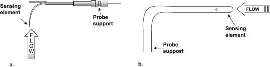
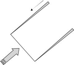
Measurement techniques can be characterized as invasive or noninvasive and direct or indirect. Invasive measurement techniques require the insertion of a sensing or a sampling element directly into the flow field. As a result of this direct insertion, invasive probes may alter the flow field characteristics or induce bias errors associated with the presence of the probe in the flow field or by the operation of the probe (11,12). Invasive probes are often designed to minimize flow disturbance by miniaturizing the sensing elements or by displacing the sensing elements some distance from the hardware holding the probe in the flow, as illustrated in Fig. 1. Invasive probes also require some type of closure at the penetration site through the boundary of the flow, which must be accounted for in the test design and can be particularly important in in vivo applications to prevent fluid loss or infection. White et al. (13) measured wall shear stress in the abdominal aorta of dogs using an invasive, flush-mounted hot-film probe and described how the probe tip is modified to provide an effective entry mechanism through the arterial wall with an adequate seal.
Noninvasive techniques do not involve direct insertion of a sensor into the flow but provide sensing capability through either access to the flow at the flow boundary or through the use of some form of electromagnetic radiation (EMR) transfer or propagation. Wall-mounted thermal sensors, static pressure taps and transducers, or surface
FLOWMETERS 323
Figure 1. Examples of invasive velocity measurement sensors with displaced sensing elements relative to their probe supports. (a) a boundary layer style hot-wire probe for thermal anemometry. Picture from TSI Inc. catalog, probe catalog 1261A. (b) Pitot static probe for velocity measurement.
sampling probes are examples of noninvasive techniques that require access to the boundary of the flow field through a wall penetration (13). Ultrasound (14) magnetic resonance (MR), X-ray, and optical techniques are all examples of electromagnetic radiation that can be used to probe flow fields (15). Unlike the wall-mounted invasive probes describe above, EMR-based measurement systems do not require physical penetration into the flow field or access through the flow field boundary. They do, however, require a ‘‘window’’ into the flow through the boundary enclosing the flow field of interest. This ‘‘window’’ depends on the type of technique being used. Optical-based techniques require an optically clear window that may not be suitable for in vivo applications, whereas ultrasound and X-ray techniques require that the material properties of the flow boundaries are transparent to these forms of EMR waves. For example, lead will shield X-ray penetration and metal objects on a surface or in the flow may create local artifacts (noise or error) in MR measurements.
Direct and indirect measurements are defined by how quantities of interest are measured. The displacement of a particle or cell in a flow can be directly measured by photographing the movement of the particle over a finite time interval (16). Most flow-related measurement systems, however, are indirect. In general, velocity or flow is indirectly calculated from the direct measurement of a quantity and the application of a calibration that relates the magnitude of the measured quantity to the parameter of interest. This calibration may involve not only a conversion of a measured quantity like a voltage to a physical quantity such as a pressure, but may also involve the application of a functional relationship (i.e., Bernoulli’s equation), which requires assumptions about the flow. For example, volume flow probes often assume a characteristic velocity profile at the location of the probe (17). Blood flow in the microcirculation can be estimated by indirectly measuring the cell velocity using a time-of-flight optical technique where the time a cell takes to move a known distance is measured and the cell velocity is calculated by the ratio of the distance divided by the transit time (18).
Indirect measurement can also impact the uncertainty in the estimated quantity. The measurement of velocity using a Pitot probe is one example of an indirect measurement (19). The Pitot probe measures the local dynamic and static pressures in the flow. These pressures are most often measured using a pressure transducer that provides a voltage output in response to an applied pressure. A cali-
bration is then applied to the measured voltage to convert it to pressure. Velocity is indirectly calculated from the estimated pressures using the Bernoulli equation. The error in Pitot probe velocity measurements includes the pressure transducer calibration uncertainty, noise and statistical uncertainty during the pressure measurement, electronic noise in the acquisition of the transducer output voltage, and transducer drift and potential bias due to the physical size of the probe relative to the flow scales being measured. These errors are nonlinearly propagated into the estimate of the velocity uncertainty.
Measurement accuracy is also a function of the physical and operating characteristics of the probe itself. Many flows exhibit a range of spatial and temporal scales. The physical size and the frequency response of the sensing element must be taken into account when choosing a measurement system for a particular application. A large sensing element or an element with poor frequency response has the effect of low pass filtering the measured signal (20). This low pass filtering will cause a bias in the measured quantity. The total measurement uncertainty must also take into account statistical errors associated with random processes, cycle-to-cycle variability in pulsatile systems, and noise. The reader is referred to the texts by Coleman and Steele (21) and Montgomery (22) for a detailed approach to experimental uncertainty analysis. The focus of this chapter will be on measurement techniques, their fundamentals of operation, their advantages and disadvantages, and examples of their use.
The name flow measurement is a broad term that can encompass the measurement of many different flowrelated parameters. In this chapter, the authors will focus on the measurement of those parameters that are most often desired in a biomedical/bioengineering application, volume flow rate, and velocity. Imaging, Doppler echocardiography, and MR techniques are addressed in other chapters within the encyclopedia and, thus, will only be briefly introduced in this article when applicable. This chapter is subdivided into sections that will address volume flow and velocity separately, with a detailed presentation of systems that are available for the measurement of each. Although ultrasound and MR techniques are often used to measure flow-related parameters, a detailed discussion of the principles of operation will not be presented here as these topics are covered in depth in other chapters of this Encyclopedia.
324 FLOWMETERS
FLOW MEASUREMENT APPLICATIONS
Volume Flow Measurement
In both the clinical environment and the laboratory environment, the measurement of the volume flow rate of a fluid as a function of time can be an important parameter. In internal flow applications, which comprise most biomedical flows of interest, the volume flow of a fluid (Q) is related to the local fluid velocity (V) through the integration of the velocity over
the cross sectional area of the duct or vessel (19,23).
ð
Q ¼ V dA |
(1) |
The flow rate Q, velocity V, and area A have dimensions of volume per time, length per time, and length squared, respectively. The SI units are typically used in the bioengineering field with mass units of grams or kilograms, length units of meters (millimeter and centimeters), and time units of seconds. The mass flow (M) is directly related to the flow volume through the fluid density, r, with units of mass/volume.
M ¼ r Q |
(2) |
Fluid pressure and velocity are related through the Navier–Stokes equations, which govern the flow of fluids in internal and external flows [see White (23)].
The volume flow rate of blood is often measured in many cardiovascular applications (24). For example, cardiac output (CO) is the integrated average of the instantaneous volume flow rate of blood (Qb) exiting the aortic valve over one cardiac cycle (Tc):
CO ¼ ð Qbdt =Tc |
(3) |
The cardiac output has units of volume flow rate, volume per unit time. The following subsections will provide an overview of measurement techniques typically used for both volume flow and velocity measurement in in vivo and in vitro studies. This article will be limited to those flow measurement techniques most often used in the biomedical and bioengineering fields. Specialized measurement techniques, such as concentration or species measurement through laser-induced fluorescence (LIF) or mass spectrometry, will not be addressed.
Electromagnetic Flow Probes. Carolina Medical Inc. developed the first commercially available electromagnetic flow meter in 1955. The design provided scientists and clinicians with a noninvasive tool that could directly measure the volume flow rate (17). Clinical probes were developed that could be attached to a vessel for extravascular measurement of blood flow without the need for cannulation of a surgically exposed vessel.
Electromagnetic flow meters are volumetric flow measuring devices designed to measure the flow of an electrically conducting liquid in a closed vessel or pipe. Commercial meters, used in the biomedical and general engineering fields, come in a variety of sizes and designs that can measure flow rates from 1 mL min 1 to >100,000 L min 1.
Reported uncertainties are typically on the order of a few percent, but can be as low as 0.5% of reading in some specialized meter designs. Low uncertainties are dependent on proper use and installation of the meter. Improper use or installation (mounting the meter in a location with a complex flow profile) will increase measurement uncertainty. Most clinical quality meters that are mounted externally to a vessel exhibit uncertainties that can approach 15% in some applications (Carolina Medical Inc., product support literature). In cardiovascular applications, these meters may also be susceptible to electrical interference by the heart or by measurement anomalies due to motion of the probe.
The principle governing the operation of an electromagnetic flow meter is Faraday’s law of electromagnetic induction. This law states that an induced electrode voltage is proportional to the velocity of flow of a conductor through a magnetic field of a known density. Mathematically, this law is represented as:
Ee ¼ K½V B Le& |
(4) |
Here, Ee is the induced voltage between two electrodes (with units of volts) separated by a known conductor length Le (provided by the conducting fluid between the electrodes) in units of millimeters or centimeters, B is the magnetic field strength in units of Tesla’s, and V is the conducting fluid average velocity in units of length per time. The parameter K is a dimensionless constant. Meter output is linear and proportional to flow velocity.
Fluid properties such as viscosity and density are absent from Eq. 4. Thus, the output of an electromagnetic flow meter is independent of these properties and its calibration is independent of the type of fluid, provided the fluid meets minimum conductivity levels. This meter can then be used for highly viscous fluids, Newtonian fluids, and nonNewtonian fluids such as blood. The requirement of an electrically conductive fluid can disqualify an electromagnetic meter in some applications. Typical meters require a minimum fluid conductivity of 1 m S/cm 1. However, low conductivity designs are capable of operating with fluid conductivities as low as 0.1 m S/cm 1. The presence of gas bubbles in the fluid can cause erratic behavior in the meter output.
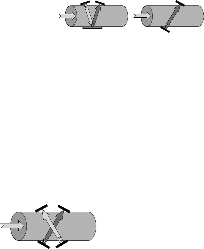
A typical meter design has electromagnetic coils mounted on opposing sides of an electrically insulated duct with two opposing electrodes mounted 908 relative to the electromagnets. The two electrodes are mounted such that they are in contact with the conducting fluid. Figure 2 illustrates the typical configuration.
The meter is designed to generate a magnetic field that is perpendicular to the axis of motion of the flowing fluid. A voltage is generated when the conducting fluid flows through the magnetic field. This voltage is sensed by the two opposing electrodes. The supporting material around the meter is made of a nonconducting material to prevent leakage of the voltage generated in the moving fluid into the surrounding material. In practice, the conductor length, Le, is not the simple path illustrated, but is rather the integral of all possible path lengths between the two electrodes across the cross section of the duct or vessel. The
|
Insulated |
Electrode |
duct |
|
|
Magnetic |
|
field |
|
|
Electro- |
|
magnet |
|
V |
|
Electrode |
Le
Conducting fluid
Figure 2. Illustration of the principle of operation of the electromagnetic flow meter. Note, the magnetic field, electrodes, and flow direction are all mutually perpendicular to one another.
signal generated along each path length is proportional to the fluid velocity across that path. Thus, the two electrodes measure the integrated sum of all velocities across every possible path in the vessel cross section. This signal is then directly proportional to the volume flow rate of the fluid passing through the magnetic field.
The magnetic field generated in commercial meters may be anything from a uniform field to a specifically designed field with prescribed characteristics. Meters with uniform magnetic fields can exhibit some sensitivity to the conducting liquid’s velocity profile. Fluid flowing through a vessel does not have the same velocity at all locations across the vessel. The no-slip condition at the walls of the duct ensures that the fluid velocity at the wall is zero (19). Viscosity then generates a gradient between the flowing fluid in the vessel and the stationary fluid at the wall. In complex geometries, secondary flows may occur and velocity gradients in other directions may also develop (25,26). This variation in fluid velocity across the magnetic field coupled with variations in the conductor length generates a variation in the magnitude of the voltage measured across the duct. As a result, installation of these meters must be carefully performed to ensure that the velocity profile of the liquid in the tube is close to that used during calibration.
A number of commercial meters shape the magnetic field coils to generate a magnetic field that exhibits a field strength with a prescribed pattern across the duct. This field shaping compensates for some velocity variations in the duct and provides a meter with a reduced sensitivity to flow profile. As a result, this type of meter is better able to measure in vessels with upstream and downstream characteristics, such as curvature and nonuniformity in the vessel cross section, that generate asymmetric flow profiles with secondary flow velocity components.
Commercial meters generate magnetic fields using either an ac excitation or a pulsed dc excitation. The ac excitation generates a magnetic field with a strength that varies with the frequency of the applied ac voltage. This
FLOWMETERS 325
configuration produces a meter with a relatively high frequency response but with the disadvantage that the output signal not only varies with the flow velocity but also with the magnitude of the alternating excitation voltage. Thus, the output of the meter for a flow with constant velocity across the vessel will exhibit a sinusoidal pattern. In addition, zero flow will produce an offset output due to the presence of the nonmoving conductor in a moving magnetic field. Quadrature signal rejection techniques can be used to filter the unwanted signal generated by the ac excitation from the desired signal generated by the flowing liquid, but this correction requires careful compensation and zeroing of the meter in the flow field before data acquisition.
The pulsed dc excitation was developed to reduce or eliminate the zero shift encountered with ac excitation. This improvement has the cost of reduced frequency response and increased sensitivity to the presence of particulates in a fluid. Particles that impact the electrodes in a pulsed dc operated meter produce output fluctuations that can be characterized as noise. The accuracy in each system is comparable.
A low sensing voltage at the electrodes requires a signal conditioning unit to provide a measurable output with a good signal-to-noise ratio. Meter calibrations typically involve one of two calibration techniques. The meter and signal conditioning unit are calibrated separately or the meter and signal conditioning unit are calibrated as a system. The latter provides the most accurate calibration with accuracies that can approach 0.5% of reading in certain applications. The reader is referred to literature by various manufacturers of electromagnetic flow meters for a more comprehensive discussion of the techniques, operation, and use for specific applications.
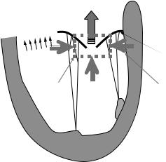
Ultrasound Techniques – Transit Time Volume Flow Meters. Ultrasonic transit time flow meters provide a direct measure of volume flow by correlating the change in the transit time of sound waves across a pipe or vessel with the average velocity of the liquid flowing through the pipe (17,27,28). Transit time ultrasonic flow meters are widely used in clinical cardiovascular applications. In recent years, a number of studies have been performed to evaluate and compare transit time ultrasonic flow measurement techniques with other techniques used clinically (29). The typical configuration for an ultrasonic flow probe involves one or two ultrasonic transducers (transmitters/ receivers) and possibly an ultrasonic reflector. Transducers and reflectors are positioned in opposing configurations across a tube or vessel as illustrated in Fig. 3. The time it takes an ultrasound wave to propagate across a fluid depends on the distance of propagation and the acoustic velocity in the fluid. If the fluid is moving, the motion of the fluid will positively or negatively add a phase shift to the time of propagation (transit time) through the fluid, which can be written mathematically as:
Tt ¼ Dp=ðc V cos yÞ |
(5) |
Here, Tt is the measured transit time (s), Dp is the total propagation distance of the wave (length units), c is the acoustic speed of the fluid (units of length per time), V is
326 |
FLOWMETERS |
|
|
|
|
Transducers |
|
|
|
Transmit |
Receivers |
|
|
Receive |
|
|
Flow |
|
Flow |
Figure 3. Illustration of principal of |
|
|
|
transit time ultrasonic flow probe |
Reflector |
|
|
operation. |
|
|
Transmitters |
the average velocity of the fluid (units of length per time) over the propagation length, and u is the angle between the flow direction and the propagation direction of the wave. The configurations illustrated in Fig. 3 have an inherent dependency of the measured transit time on the coupling of the transducer with the vessel. Acoustic impedance characteristics of the vessel wall, and mismatches in impedance at the vessel wall–transducer and wall–fluid interfaces will affect the accuracy of the flow rate measurement.
The approach to using equation 5 in a metering device is to incorporate bidirectional wave propagation in opposing directions, as shown in Fig. 4, which will produce two independent transit time measurements (Tt1 and Tt2), one from each direction of propagation. The forward direction transit time Tt1 is defined by Eq. 5 with a plus sign before V, and Tt2 is defined by the minus sign. The fluid velocity can then be obtained by taking the difference of the transit times (Tt1 Tt2). It can be shown that, for fluid velocities small relative to the acoustic velocity of the fluid (V2 << c2), this difference reduces to:
ðTt1 Tt2Þ ¼ 2 DpðV cos yÞ=c2 |
(6) |
With the probe geometry defined (the propagation distance and propagation angle relative to the vessel or flow direction) and with the fluid properties known (acoustic speed of the fluid), the average speed of the fluid along the propagation path of a narrow beam can be calculated from the transit times. Wide beam illumination, where the beam width is wider than the vessel diameter, effectively integrates the measured transit time phase shift over the cross section of the vessel. The wide beam transmission can be approximated by the summation of many infinitesimally narrow beams adjacent to one another. Thus, the measured
Receivers
Flow
Transmitters
Figure 4. Bidirectional wave propagation.
wide beam phase shift is proportional to the sum of these narrow beams propagating through the vessel. As the phase shift encountered in a narrow beam transmission is proportional to the average fluid velocity times the beam path length, integrating or summing over all narrow beams across the vessel results in a measured total transit time phase shift that is proportional to the average fluid velocity times the area of the vessel sliced by the ultrasound beam, or the volume flow rate.
The popular Transonic Systems Inc. flow meter uses bidirectional transmission with two transducers operating in transmit and receive modes, and a single reflector configured as illustrated in the left schematic of Fig. 4. This approach increases the propagation length while effectively reducing sensitivity to wall coupling or misalignment of the probe with the wall. The increased path length improves uncertainty and provides a probe body with a relatively small footprint, an advantage in in vivo or surgical applications.
The basic operation of a bidirectional transit time meter involves the transmission of an ultrasound plane wave at a specific frequency. This wave propagates through the vessel wall and fluid where it is either received at the opposite wall or is reflected to another transducer operating as an acoustic receiver. This received signal is recorded, processed, and digitized before the transducer is reconfigured to transmit a second pulse in the opposite direction. The overall frequency response of such a probe is dependent on the pulse time, the time delay between the forward and reverse pulses, the acoustic speed through the medium, the propagation distance, and the signal conditioning electronics, which can include analog signal acquisition and filtering. The meter size governs the propagation distance and, thus, the size of the vessel that the meter can be mounted on.
The frequency response of commercial probes varies from approximately 100 Hz to more the 1 kHz, where the highest frequency responses are obtained in the smaller probes. As a result, commercial probes have sufficient frequency response for most clinically or biomedically relevant flow regimes. Velocity and flow resolution is governed, in part, by the propagation length over which the flow is integrated and the resolution of the transit time measurement. The reader is referred to the meter manufacturers for detailed information about the operating specifications of particular meters. Reported uncertainties in transit time meters can be better than 15%. Actual uncertainties will depend on meter use, the experience of the operator, the meter calibration, and the acoustic properties of the
FLOWMETERS 327
Doppler transducer
Increased frequency of scattered beam
Flow
Reflectors
Figure 5. Schematic of the operation of a Doppler ultrasound probe.
fluid measured and how these properties differ from those of the calibration fluid.
Ultrasound Techniques – Doppler Volume Flow Meters.
Flow can also be measured by ultrasound using the Doppler shift in a propagating sound wave generated by moving objects in a fluid flow (17,30). The primary difference is in the principal of operation. Devices using the Doppler approach measure the Doppler frequency shift of the transmitted beam due to the motion of particles encountered along the beam path, as illustrated in Fig. 5. The Doppler shift due to reflection of an incident wave by a moving particle is given by
FD ¼ 2 Fo V cos y=c |
(7) |
The shift frequency FD (units of L s 1) is linearly related to the component of the speed of a particle, V, in the direction of the wave propagation, the initial transmission frequency of the wave, Fo, and the speed of sound in the fluid, c. The reader is referred elsewhere in this Encyclopedic series and to the text by Weyman (30) for a detailed presentation of the Doppler technique.
The Doppler meter provides a direct measure of velocity that can be used to calculate the volume flow rate indirectly. Most biomedical applications involving volume flow measurement are performed on flow through a duct or vessel of given shape and size. Thus, the volume flow is the integral of the measured velocity profile across the vessel cross sectional area as defined in equation 1. The integral in equation 1 can be related to the average velocity
¯ across the duct multiplied by the cross-sectional area of
U
the duct (23). The Doppler technique then requires not only an estimate of the average velocity in the vessel but knowledge of the vessel area as well.
Commercially available Doppler volume flow meters, although not commonly used in biomedical applications, can be attached to a pipe or duct wall as with transit time meters. The commercial Doppler flow meters measure volume flow by integrating the measured Doppler shift frequency generated by particles throughout the flow. This integration is performed over a predefined path length in the flow, and is dependent on the number and type of particles, their size and distribution. The meter accuracy
is also dependent on the velocity profile in the flow. Careful in situ calibrations are often needed to obtain accuracies of less than 10%. The Doppler meter has several disadvantages when compared with the transit time meter. It requires a fluid that contains a sufficient concentration of suspended particles to act as scattering sites on the incident ultrasound wave. These particles must be large enough to scatter the incident beam with a high intensity level but small enough to ensure that they follow the fluid flow (31). As a result of their dependence on flow profile, Doppler flow meters are not well-suited for measurement of flow in vessels with curvature or branching. Doppler flow meter measurements in blood rely on blood cells to act as scatterers. Clinical Doppler ultrasound machines, commonly used in echocardiography, can also be used to indirectly infer volume flow through the direct measure of the fluid velocity, and will be discussed later in the subsection on velocity measurements.
Invasive or Inline Volume Flow Measurement. Invasive or inline flow meters must be installed inline as a part of the piping or vessel network and involve hardware that is in contact with the fluid. These meters often have a nonnegligible pressure drop and may adversely interact with the flowing fluid. As a result, these meters are not often used in in vivo applications. Meters that fall in this category are variable area rotameters, turbine/paddle wheel meters, and vortex shedding meters. The primary advantage of these meters, is low cost and ease of use. However, these meters typically exhibit sensitivity both to fluid properties, which can be dependent on temperature and pressure, and to flow profile, White (23).
Variable area rotameters are simple measurement devices that can be used with a variety of liquids and gases. The flow of fluid through the meter raises a float in a tapered tube, as shown in Fig 6. The higher the float is raised, the larger the diameter of the tapered tube, increasing the cross-sectional area of the tube for passage of the fluid. As the flow rate increases, the float is elevated higher in the tube. The height of the float is directly proportional to the fluid flow rate. In liquid flow, the float is raised by the combination of the buoyancy of the liquid and the fluid drag on the float. Buoyancy is negligible in gaseous flows
328 FLOWMETERS
Gravity
S
C
A
L
Q E
Figure 6. Schematic of a variable area flowmeter.
and the float moves in response to the drag by the gas flow. For constant flow, the float reaches a stable position in the tube when the upward force generated by the flowing fluid equals the downward force of gravity. The float will move to a new equilibrium position in response to a change in flow. These meters must be installed vertically to operate properly, although spring-loaded meters have been designed to eliminate the need for gravity and permit installation in other orientations.
Rotameters are designed and calibrated for the type of fluid (fluid properties such as viscosity and density) and flow range expected. They do not function properly in nonNewtonian fluids. Use of a meter with a fluid different from that the meter was calibrated for, or with, a fluid at a different temperature or pressure requires a correction to the meter reading. Meter uncertainty and repeatability will vary with operation of the meter, but can approach a few percent with proper operation.
Turbine and paddle wheel meters measure volume flow rate through the rotation of a vaned rotor in contact with the flowing fluid. These meters are intrusive flow measurement devices that produce higher pressure drops than others in the class of invasive flow probes. The turbine meter has a turbine mounted across the pipe or duct in full contact with the flow, whereas the paddle wheel meter has a vaned wheel mounted on the side of the duct with half of the wheel in contact with the flow. Accuracy and repeatability is best with the turbine meter, but the pressure drop is also higher. An ac voltage is induced in a magnetic pickup coil as the turbine or paddle wheel rotates. Each pulse in the ac signal represents the passage of one blade of the turbine. As the turbine fills the flow path, a pulse represents a distinct volume of fluid being displaced between two turbine blades. This design provides an accurate direct measure of the volume flow rate.
Flowmeter selection must take into account the type of fluid, the flow rate range under study, and the acceptablepressure drop for a given flow application. In general, these meters have a sensitivity to flow profile, and the pressure drop is dependent on the fluid properties. The meters incorporate moving parts within the flow and thus use bearings to ensure smooth operation. Bearing wear will affect the meter accuracy and must be monitored for the life of the meter. The paddle wheel meter operates in a similar manner as the turbine meter. The primary difference is that only part of the rotor is in contact with the fluid and, thus, as the paddle wheel meter is more sensitive to flow profile it has a smaller pressure drop. Installation of these
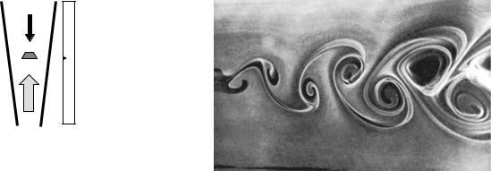
Figure 7. Vortex shedding from a circular cylinder. Picture from White (23), courtesy of the U.S. Naval Research Laboratory.
meters often involves a specified number of straight pipe sections upstream and downstream of the meter and may also require installation of a flow straightener inline upstream of the meter.
Vortex meters operate on the principal of Strouhal shedding. Separating flow over an obstruction such as a cylinder or sharp-edged bar results in a pulsatile or oscillatory pattern as shown in Fig. 7. The shedding frequency, o (units of L s 1), is related to the fluid velocity by
o ¼ V St=L |
(8) |
where St is the Strouhal number, which is a nondimensional number that is a function of the flow Reynolds number and geometry of the obstruction, and L is a characteristic length scale (23). For a cylinder, L is the diameter of the cylinder. The Reynolds number is a dimensionless number that is the ratio of inertial to viscous forces in the flow, and is defined as
Re ¼ V L=u |
(9) |
Here, V and L are defined as in Eq. 8 and u is the kinematic viscosity of the fluid with units of length squared per time.
The vortex meter is an intrusive meter that has a ‘‘shedder bar’’ installed across the diameter of the duct. The flow separates off this bar and generates a shedding frequency that is transmitted through the bar to a piezoelectric sensor attached to the bar. The meter is sensitive to flow and fluid properties, and rated accuracy and pressure drop depend on application.
Volume flow rate can also be estimated through an indirect measure of the velocity profile in the flow and the use of Eq. 1. A number of instruments are available that measure fluid velocity in biomedical engineering applications. Doppler ultrasound and MR phase velocity encoding are standard clinical techniques used to measure velocity of a flowing fluid noninvasively. In vitro systems that are commonly used to measure fluid velocity, in addition to Doppler and MR, are laser Doppler velocimetry (LDV), particle image velocimetry (PIV), and thermal anemometry. Besides an estimate of volume flow rate, fluid velocity measurement can provide quantification of flow profiles, fluid wall shear, pressure gradient, and flow
mixing. The following section summarizes velocity measurement techniques commonly used in biomedical/bioengineering applications.
Velocity Measurements
Thermal Anemometry. Thermal anemometry is an invasive technique used to measure fluid velocity or wall shear. A heated element is inserted into the flow, and specialized electronic circuitry is used to measure the rate of change in heat input into the element in response to changes in the flow field (32). Thermal anemometry, when used properly, is characterized by high accuracy, low noise, and high spatial and temporal resolution. Its main disadvantages are sensitivity to changes in fluid temperature and properties, particulates and bubbles suspended in a fluid, nonlinear response to velocity, and its invasive characteristics (geometry, size, vibration, etc.).
Hot-film anemometry has been used to measure blood velocity and wall shear in biomedical and bioengineering applications both in vitro and in vivo. Arterial blood flow velocity measurements were performed by Nerem et al. (33,34) in horses and by Falsetti et al. (35) in dogs. Tarbell et al. (36) used flush-mounted hot films to measure wall shear in the abdominal aorta of a dog. In vitro applications of hot-film anemometry include the measurement of wall shear in an LVAD device (37), and the in vitro measurement of flow in rigid models of arterial bifurcations by Batten and Nerem (38). Although rarely used in biomedical applications now, we will briefly present hot-film anemometry here for completeness. The reader is referred to the text by Bruun (39) and the symposium proceedings by Stock (40) for a detailed presentation of thermal anemometry.
Thermal anemometry operates on the principal of convective cooling of a heated element. A thin wire or coated quartz element, mounted between supports, is heated and exposed to a fluid flow, as shown in Fig. 8. The element is heated by passing a current through the wire or element. The amount of heat generated is proportional to the current, I (A), and the resistance of the element, R (V), by I2R. The element is convectively cooled by flow until an equilibrium state is reached between electrical heating of the
I
Supports
Wire or film
Q
Figure 8. Illustration of a hot wire or film element.
FLOWMETERS 329
element and flow-induced convective cooling, DE/ Dt ¼ W þ H, where E is the thermal energy stored in the element, W is the heat added by joule heating, and H is the heat loss to the environment by cooling. At equilibrium,
DE/Dt ¼ 0 and W ¼ H.
Changes in flow velocity will increase or decrease the amount of convective cooling and produce changes in the equilibrium state of the element or the temperature of the element. Commercial anemometers employ a four-arm electronic bridge circuit to maintain constant element temperature, current, or voltage in response to changes in convective cooling. As convective cooling changes, the anemometer output, current, or voltage changes in response to maintaining the desired set condition. This equilibrium condition assumes that radiation losses are small, conduction to supports is small, temperature is uniform over length of sensor, velocity impinges normally on the sensor, velocity is uniform over sensor length and is small compared with the sonic speed, and finally, the fluid temperature and density are constant.
An energy balance between convective heat cooling and joule heating can be performed to derive a set of governing equations that relate input current, I, to convective velocity, V. The ‘‘King’s law’’ is the classic result of this energy
balance: |
|
I2R2 ¼ Vo2 ¼ ðTw TaÞðA þ B VnÞ |
(10) |
where Vo is the measured voltage drop in response to a velocity, V, and Tw and Ta are the wire and ambient fluid temperatures (8C), respectively. The coefficients, A and B, and power, n, are determined through careful calibration over the velocity and temperature range that will be observed experimentally. In the event of a three-compo- nent flow, the probe must be calibrated for yaw and pitch angles between the probe and the flow velocity vector, and the velocity, V, in Eq. 10 must be replace by a term related to the velocity vector magnitude. Bridge-type circuits are also prone to stable and unstable performance under unsteady operation. Thus, the overall calibration of a hot-wire/film system must involve the element and electronics as a system and must also involve dynamic calibrations to characterize the frequency response of the system.
Hot-wire/film probes come in a variety of sizes, shapes, and configurations. Probes are manufactured from platinum, gold-plated tungsten, or nickel-plated quartz, and come in single-element or multielement configurations for measurement in a variety of flow conditions. The reader is referred to the hot-wire/film manufacturers for a complete summary of probe types and conditions for use. In general, wire probes are used when possible due to lower cost, improved frequency response, and ease of repair. However, wire probes are more fragile compared with film-type probes and are usually restricted to air flows. Film probes are used in rough environments, such as liquid flows.
The following considerations should be addressed to ensure accurate measurements when using thermal anemometry. The type of flow should be assessed for velocity range, flow scales, and fluid properties (clean gas or particle contaminated liquid, etc.). The flow characteristics will define the right probe, anemometer configuration, and
330 FLOWMETERS
A/D setup to use. Perform appropriate calibrations with complete hardware setup. Perform the experiment and post calibrations to ensure that the anemometer/probe calibration has not changed.
Doppler Ultrasound And Magnetic Resonance Flow Mapping. The focus of this subsection is to introduce the concept of Doppler ultrasound and MR flow mapping for local velocity measurement. Flow measurement using clinical Doppler can suffer from the same limitations as the small Doppler meter, but has several advantages over these small meters. Most ultrasound machines can operate in continuous wave or pulsed Doppler modes of operation; see Weyman (30) for a more detailed discussion of the modes of operation.
Pulsed Doppler ultrasound offers the advantage of localizing a velocity measurement within a flow and can be used to measure the velocity profile across a vessel or lesion. This information coupled with echocardiographic imaging of the geometry can be used to calculate the flow rate from Eq. 1. Unfortunately, the implementation of this technique is not straightforward due to limitations in resolution, velocity aliasing, and the need to know the relative angle between the transmitted ultrasound beam and the local flow.
Velocity aliasing in pulsed-mode Doppler occurs because the signal can only be sampled once per pulse transmission (e.g., the pulse repetition frequency). Frequency aliasing, or the ambiguous characterization of a waveform, occurs in signal processing when a waveform is sampled at less than one-half of its fundamental frequency, referred to as the Nyquist condition in signal processing. In a pulsed Doppler system, velocity aliasing will occur when the Doppler shift of the moving particles exceeds half of the pulse repetition frequency. As the pulse repetition frequency is a function of the depth at which a sample is measured, the alias velocity will vary with imaging depth. Increasing the imaging depth will lower the velocity at which aliasing will occur. Continuous wave Doppler signals are typically digitized at higher sampling frequencies, limited by the Nyquist frequency associated with the frequency of the transmission wave. Velocities observed clinically produce Doppler shifts that are generally lower than sampling frequencies used in continuous wave Doppler. As a result, velocity alias is not usually observed with continuous mode Doppler in clinical applications.
Aliased signals that are processed by the measuring system are not directly proportional to the Doppler shift generated by the velocity of the particle but can be related to the Doppler shift. Undersampling a wave underestimates the frequency and produces a phase shift. Most clinical Doppler machines use the frequency and phase of the sampled wave to infer velocity magnitude and direction. Velocity alias will produce a lower velocity magnitude with increasing Doppler shift above the alias limit. As frequency is, by definition, positive and Doppler machines use the signal phase to determine direction, the measured frequency is usually reported as a negative velocity above the alias limit, which is often displayed as an increasing positive velocity magnitude with increasing Doppler shift up to the alias limit. Further increases in the Doppler shift
(particle velocity) result in a sign change at the velocity magnitude of the alias velocity with a continued decrease in velocity with increasing Doppler shift. Velocity alias can be reduced or eliminated by frequency unwrapping and baseline shifting, or through the careful selection of machine settings during data acquisition.
Frequency unwrapping is simply correcting the reported aliased velocity by a factor that is related to the alias velocity limit and the magnitude of the reported negative velocity. This correction is, roughly speaking, adding the relative difference in magnitude between the measured aliased velocity and the velocity alias limit to the velocity alias limit. This method of addressing velocity alias is often accomplished by baseline shifting in commercial Doppler machines. In baseline shifting, the phase angle at which a negative velocity is defined is shifted with the effect of a relative shift in the reported alias velocity. Baseline shifting or frequency unwrapping does not eliminate velocity alias but provides a correction to extend the measurement to higher frequencies.
Velocity alias can be ‘‘eliminated’’ by reducing the Doppler frequency of moving particles and thereby shifting the measurable range below the alias limit, which can be accomplished by reducing the carrier frequency of the ultrasound wave that will, in turn, reduce the Doppler frequency shift induced by a moving particle and increase the maximum velocity that can be recorded before reaching the Nyquist limit. Alternatively, the Doppler shift frequency can be reduced by increasing the angle between the propagation of the ultrasound wave and the velocity vector, which reduces the magnitude of the Doppler shift frequency by the cosine of this included angle. Angle correction has limitations in that the flow direction must be known and the uncertainty in the correction increases with increasing included angle. As color flow mappers operate in the pulsed Doppler mode, they are subject to velocity alias. Color flow mappers indicate velocity direction by a color series (for example, shades of red or blue). Velocity alias is displayed as a change in a color series from red-to-blue or blue-to-red.
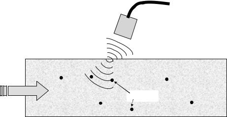
The clinical measurement of many velocity ensembles across a vessel and the integration across the vessel geometry can be time-consuming and problematic in pulsatile flow through a compliant duct. Furthermore, lesions are often complex in shape and cannot be adequately defined by echo. Doppler echocardiographers and scientists have exploited the physics of fluid flow to develop diagnostic tools that complement these capabilities of commercial Doppler systems. The text by Otto (41) provides an excellent review of these diagnostic tools. Techniques such as the PISA or proximal flow convergence use the capability of color Doppler flow mapping machines to estimate volume flow through an orifice, such as a heart valve. Figure 9 illustrates the concept of the proximal flow convergence method.
The flow accelerating toward a small circular orifice will increase in velocity Va, until a maximum velocity at the orifice Vj is reached. This acceleration occurs in a symmetric pattern around the orifice and is characterized by hemispheres of constant velocity. As the orifice is approached, the velocity increases and the radius of the
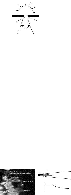
Va
|
|
Accelerating proximal flow |
Regurgitant jet |
Vj |
Heart valve lesion |
|
|
|
orifice velocity |
|
|
Figure 9. Illustration of the proximal isovelocity surface area (PISA) concept.
hemisphere decreases. The regurgitant flow through the orifice can then be calculated as:
Q ¼ ð2pr2ÞVa |
(11) |
The combined imaging and Doppler characteristics of color Doppler flow mapping are exploited in the PISA approach. The location of the alias velocity in the flow map provides a measure of Va, which is then coupled with a measure of the radial location from the orifice using the imaging capability of color flow mapping. As flow is velocity times area, the hemispheric assumption provides a shell with a surface area of 2pr2 that velocity Va is passing through. Figure 10 illustrates the concept of PISA with a color Doppler flow image of valvular regurgitation in a patient.
The PISA approach assumes a round orifice with a hemispherical acceleration zone. In clinical applications, orifices are rarely round and the acceleration zone is not hemispherical with the result of under or over estimation of the flow rate depending on what radial velocity contour is used in Eq. 11. The semielliptic method is one approach at considering nonhemispheric geometries in an attempt to correct for errors associated with the PISA technique.
The combination of continuous wave and pulsed Doppler ultrasound is exploited in the turbulent jet decay method of measuring flow through a stenotic lesion or a regurgitant valve. While continuous wave Doppler does not suffer from velocity alias as does pulsed Doppler, it cannot provide spatial localization of the velocity. The turbulent
|
|
|
|
|
Potential |
|
|
|
|
|
|
Jet Core |
|
|
|
|
|
|
Vj = Vj max |
|
|
|
|
Vj MAX |
|
|
|
|
iso-velocity contour measured |
|
|
|||
|
by color Doppler flow mapping |
|
|
|
Vj (x) |
|
|
|
|
||||
|
|
|
|
|
|
|
|
valve lesion |
|
|
|
|
|
|
|
|
|
|
|
|
|
|
|
|
Vj |
|
|
(a) |
|
(b) |
|
x |
||
|
|
|
||||
Figure 10. (a) Color Doppler flow map image of the proximal isovelocity surface area (PISA) in valvular regurgitation.
(b) Illustration of the jet decay downstream of an orifice. The parameter V is the jet velocity and x is measured from the orifice.
FLOWMETERS 331
jet decay method uses continuous wave Doppler to measure the high velocity at the lesion orifice and then uses pulsed Doppler to measure the velocity decay at specified location downstream of the orifice. Turbulent jet theory can be used to relate the flow rate of the turbulent jet to the decay of the jet velocity downstream of the orifice, as in Eq. 12
Q ¼ ðpVm2 x2Þ=160 Vj |
(12) |
The velocity Vm is measured by pulsed Doppler at location x measured from the jet orifice, whereas the orifice velocity, Vj, is measured by continuous wave Doppler; Fig. 10b illustrates this decay phenomenon. This equation is valid for round jets and has been extended to jets with other geometries by Cape et al. (42) with the resulting change to Eq. 12:
Q ¼ ðVm2 HxÞ=5:78 Vj |
(13) |
where H is the width of the jet measured by color Doppler. Doppler velocity measurements are also used to estimate pressure gradients in various cardiovascular applications. The Bernoulli equation can be used to estimate the pressure drop across a stenotic lesion or through a valve by measuring the velocity both upstream and downstream of
the lesion or valve. The Bernoulli equation is
DP ¼ ðP1 P2Þ ¼ 1=2 rðV22 V12Þ
where position 1 is often measured upstream of the lesion and position 2 is at the lesion or downstream. In this equation, the pressure drop DP has units of Pascal’s (Pa). A Pascal is a Newton (N) per square meter, where a Newton has units of mass (kg) times length (meter) per time squared. Bioengineering and biomedical applications often use the units of millimeters of mercury (mmHg) in defining a pressure value. A mmHg is related to a Pa by the conversion; 1 mmHg ¼ 133.32 Pa.
Magnetic resonance flow mapping has the advantage over Doppler that it can measure the full three-component velocity field over a volume region (43–45), which eliminates the uncertainty in flow direction and enables the use of standard fluid dynamic control volume analysis. The advantages of MR flow mapping come at the cost of long imaging times and increased sensitivity to motion artifacts in in vivo applications, where phase locking to the heart rate or breathing cycle can increase complexity.
The velocity of moving tissue can be detected by a time- of-flight technique (46) and by phase velocity encoding (47,48). The time-of-flight method tracks a selected number of protons in a plane and measures the displacement of the protons over a time interval defined by the imaging rate. In vivo (49) and phantom (50) studies have shown that the time-of-flight technique is capable of accurate velocity measurement up to velocities at least as high as 0.5 m s 1. However, the time-of-flight method requires a straight length of vessel on the order of several centimeters for accurate velocity estimation. This requirement reduces its usability in most in vivo applications. The phase velocity encoding method has become the preferred technique in most clinical applications.
Phase velocity encoding directly relates the local velocity of nuclei to the induced phase shift in an imaging voxel.
332 FLOWMETERS
Properly defined bipolar magnetic field gradients are produced in the direction of interest for velocity measurement. The velocity of hydrogen nuclei are then encoded into the phase of the detected signal (51). Chatzimavroudis et al. (52) and Firmin et al. (53) provide a discussion of the phase encoding technique with an assessment of its accuracy and limitations for flow measurement.
The technique uses two image acquisitions to provide velocity compensation and velocity encoding. Velocity information in each voxel is obtained by a voxel-by-voxel subtraction of the two images with respect to the phase of the signal. Like Doppler ultrasound, phase velocity encoding can suffer from aliasing effects, alignment error, and limits in spatial and temporal resolution. Velocity estimation using phase shift measurement is limited to a maximum range of phase of 2p radians without ambiguity or aliasing. However, the estimation of the phase shift using phase subtraction between two images reduces that sensitivity to this problem. Studies have been conducted that show MR phase velocity encoding can measure velocities covering the complete physiologic range up to several meters per second (54). Misalignment of the flow direction with the encoding direction will produce a negative bias in the measured flow where the measured velocity will be lower than the true velocity. Like Doppler, this bias follows
a cosine behavior where Vmeas ¼ Vact cos(u), where Vmeas is the measured velocity, Vact is the actual velocity, and u is
the misalignment angle. This error is typically less than 1% in most applications.
The size of a voxel and the sampling capabilities of the hardware characterize the spatial and temporal resolution of the system. Spatial resolution affects the size of a flow structure that can be measured without spatially filtering or averaging the structure or velocity measurement. Spatial velocity gradients that are small relative to the voxel size will not be adequately resolved and will be averaged over the voxel volume (55). In addition, rapidly varying velocity fluctuations in time will produce a similar low pass frequency filtering effect if these fluctuations occur with a time scale that is much smaller than the imaging time scale of the measurements. Turbulent flow can produce spatial and temporal scales that could be small relative to the imaging characteristics and can result in what is referred to as signal loss in the image (56). Stenotic lesions and valvular regurgitation are clinical examples where turbulent flow can occur with spatial and temporal scales that could compromise measurement accuracy.
Phase velocity encoding has the drawback of fairly long imaging or magnet residence times, which is particularly true for three-component velocity mapping. Although this may be acceptable for in vitro testing with flow loop phantoms, it can present problems and concerns with clinical measurements. Patients can be exposed to long time intervals in the magnetic with the associated problems of patient comfort and care. In vivo velocity measurements are often phase-locked with cardiac cycle or breathing rhythm. Long imaging times can increase potential for measurement error due to patient movement and variability in the cardiac cycle or breathing rhythm, which can cause noise in the phase-averaged, three-component velocity measurements. Research, in recent years, has focused
on hardware and software improvements to increase spatial resolution and reduce imaging time [see, e.g., Zhang et al. (57)].
Magnetic resonance phase velocity encoding provides coupled 3D geometric imaging using traditional MR imaging methods with three-component velocity information. This coupled database provides a powerful diagnostic tool for blood flow analysis and has been used extensively in in vitro and clinical applications. Jin et al. (6) used this coupled imaging flow mapping capability to study the effects of wall motion and compliance on flow patterns in the ascending aorta. Standard imaging was used to measure aortic wall movement and the range of lumen area and diameter change over the cardiac cycle. This aortic wall motion was phase-matched with phase velocity encoded axial velocity distributions in the ascending aorta. Similar to the PISA approach in Doppler ultrasound, a control volume approach using phase velocity encoded MR velocities can be applied to the assessment of valvular regurgitation (58,59). The control volume approach is illustrated in Fig. 11.
Laser Doppler Velocimetry. The Doppler shift of laser light scattered by particles or cells in a fluid is the basis of laser Doppler velocimetry (LDV). Detailed presentations of the LDV technique are provided in the works by Drain (60) and Durst et al. (61). The scattered radiation, from a laser beam directed at moving particles in a fluid, has a Dopplershifted frequency defined as:
fD ð1 V=C1Þ f 0 |
(14) |
where Cl is the speed of light in a vacuum, V is the particle velocity, and f 0 is incident light frequency. The Dopplershifted frequency is very small relative to the frequency of
Qr
Aortic outflow
V1 |
|
Mitral valve |
CV |
V2 |
V3 |
Figure 11. Illustration of the control volume method in MR phase velocity assessment of valvular regurgitation. The control volume (CV) is the heavy dotted line box around the mitral regurgitant orifice. The box edges are usually selected to correspond with rows and columns in the MR image. Vi represents the three-component velocities measured with MR through the i faces of the box. Faces 4 and 5 are in the plane of the image at Z offsets from the plane of the image. The regurgitant flow Qr is the sum of the ViAi on each face.
FLOWMETERS 333
Flow w/ particles
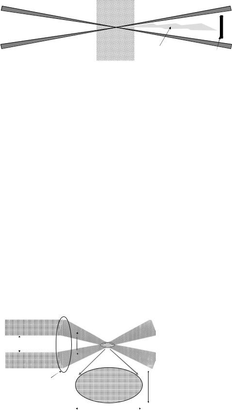
2 coherent laser beams
Scattered light
Photo |
Figure 12. Illustration of the dual- |
detector |
beam or fringe mode LDV setup. |
light and, thus, dual-beam or fringe mode LDV is the system configuration of choice. The dual-beam mode of operation is schematically shown in Fig. 12. In fringe mode LDV, two coherent laser beams of the same wavelength or frequency are focused to a common point (control volume) in the flow field. The scattered light from a particle moving through the control volume is received by a photodetector.
The crossing of two coherent, collimated laser beams forms interference fringes as the propagating light waves constructively and destructively interfere with one another. This interference creates a series of light and dark bands with spacing, df, of
df ¼ l=2 sinðkÞ |
(15) |
The number of fringes, NFR, in the measurement volume is given by
NFR ¼ 1:27d=De 2 |
(16) |
where d is the spacing between the two parallel laser beams before the focusing lens and De 2 is the beam diameter before the lens. Figure 13 illustrates the probe geometry generated by the intersection of two focused coherent laser beams with a common wavelength.
The spatial resolution of a dual-beam system is affected by the distribution of the light intensity at the intersection of the two focused beams, referred to as the probe or measurement volume. When the laser is operating in the TEMoo mode, the laser cavity sustains a purely longitudinal standing wave oscillation along its axis with no transverse modes. The laser output has an axisymmetric intensity profile that is approximately a Gaussian function
2 coherent laser beams |
2κ |
Focusing |
|
|
|
lens |
|
|
Dm |
|
|
|
|
|
lm |
|
|
Figure 13. Illustration of the measurement volume generated in fringe mode LDV.
of radial distance from the axis. In the far field, the beam divergence is small enough to appear as a spherical wave from a point source located at the front of the lens. A lens is used to focus the beam into a converging spherical wave. The radius of this wave decreases until the focal point of the lens is reached. At the focal point, the beam has almost a constant radius and planar behavior. The beam is focused to its minimum diameter or focal waist, de 2, and is defined as:
de 2 ¼ ð4l f Þ=ðpDe 2Þ
where l is the wavelength of the laser beam and f is the focal length of the lens. A single pair of laser beams generates an ellipsoidal geometry having dimensions of major axis lm and minor axis dm given by
lm ¼ de 2=sinðkÞ and dm ¼ de 2=cosðkÞ |
(17) |
where k is the half angle between the two laser beams, as illustrated in Fig. 13.
The particle velocity is calculated by the fluctuating light intensity collected by the receiver as the particle passes through the measurement volume and scatters light from the fringes. The intensity change of the scattered light from the light and dark fringes is converted into an electrical signal by a photomultiplier tube (PMT). The electrical signal represents an amplitude-modulated sine wave, with frequency proportional to the Doppler frequency shift (fD) of the particle traveling through the measurement volume. The particle velocity is then equal to the Doppler frequency multiplied by the fringe spacing. In a two-beam LDV system, the measured velocity component is in the plane of the two laser beams and in the direction perpendicular to the long axis of the measurement volume.
Coherent laser beams with the same frequency produce stationary fringes. A particle moving in either direction across the fringes will produce the same frequency independent of sign, such that a stationary fringe system can only determine the magnitude of the velocity, not the direction. To avoid this directional ambiguity, one of the laser beams of a beam pair is shifted to a different frequency, using a Bragg cell, to provide a moving fringe pattern. One laser beam from each beam pair passes through a transparent medium such as glass, in which acoustic waves, generated by a piezoelectric transducer, are traveling. If the angle between the laser beam and the acoustic waves satisfies the Bragg condition, reflections from successive acoustic wave fronts reinforce the laser beam. The beam exits at a higher frequency and a prism
334 FLOWMETERS
directs the beam to its original direction. The Bragg shift causes the fringes in the probe volume to move at a constant speed in either the positive or negative direction relative to the flow. The measured frequency by the PMT and processor is then the sum or difference of the Bragg cell frequency (typically 40 MHz) and the Doppler shift frequency. This measured frequency is then downmixed with a frequency that is a percent of the Bragg frequency (called the shift frequency) producing a frequency that has a zero shifted to a higher baseline frequency (usually on the order of several MHz). This zero shift eliminates directional ambiguity in LDV signal processing.
Laser Doppler velocimetry has excellent spatial and temporal frequency response compared with most other measurement systems. It is considered a gold standard measurement technique in biomedical applications and is the noninvasive measurement system of choice for turbulence measurements. Two disadvantages of LDV worth noting are (1) LDV noise and (2) velocity bias. The LDV is noisy when compared with other turbulence measurement systems, such as thermal anemometry, due to the use of photomultiplier tubes. These optical detectors, used for their sensitivity and high frequency response, suffer from higher noise floors than other photo detectors.
Velocity bias is a result of the random sampling characteristics of LDV. As a velocity ensemble is randomly recorded when a particle passes through a probe volume, the statistics of the measured velocity ensembles are not independent of the particle velocity. A greater number of higher speed particles will cross the measurement volume over a specified time than will slower speed particles. Standard ensemble averaging will produce mean velocity estimates that are biased toward higher velocities. This velocity bias can have a significant impact on the velocity statistics, particularly in turbulent flow. In addition to velocity bias, two other biases may occur, fringe bias and gradient bias.
Fringe bias is an error that is minimized by frequency shifting. This type of bias is created by not having enough fringe crossings to satisfy processor validation criteria when calculating a velocity, which occurs when a particle crosses the edge of the probe volume or if the particle velocity is nearly parallel to the fringes. Thus, velocity ensemble averages weight velocities from particles traveling near the center of the measurement volume or those particles that cross more fringes then others. By frequency shifting with a fringe velocity at least two times greater than the flow velocity, particles moving parallel to the fringes can cross the minimum number of fringes for validation by a processor.
Gradient bias results from a nonnegligible mean gradient across the probe volume. This bias depends on the fluid flow and the measurement volume dimensions. The mean velocity and the odd order moments are the only statistics affected by gradient bias. In general, LDVtransmitting optics are chosen to provide as small a measurement volume as possible to increase spatial resolution and reduce gradient bias. As the LDV measurement volume is longer than it is wide, experiments should be designed to ensure that the LDV optical setup is oriented to position the measurement volume diameter in the direction of the maximum gradients in the flow.
Several post processing techniques have been developed to reduce velocity bias. The recommended technique is to use a transit time weighting when computing the velocity statistics. This transit time weighting approximates the ensemble average as a time average. The reader is referred to Edwards (62) for a detailed discussion of the transit time technique and its implementation in LDV data processing.
Multiple pairs of laser beams with different wavelength (color) or polarization can be used to produce a multicomponent velocity measuring system. Two or three laser beam pairs can be focused to the same point in the flow. Each beam pair can then be used to independently measure a different component of the velocity vector. As more than one particle can pass through a measurement volume at one time, it is possible to get valid velocity component estimates from different particles. The ellipsoidal geometry of the measurement volumes exaggerates this problem. As a result, LDV data are often processed in one of two modes, random and coincident.
Random mode processing records every valid velocity ensemble as it arrives at the measurement volume, which can generate uneven sample distributions in the different velocity components or LDV channels being measured. Random mode processing has a negligible impact on mean velocity statistics but can be detrimental to turbulence estimates. Coincident mode processing uses hardware or software filters to ensure that each velocity component ensemble is measured from the same particle. Filters are used to ensure that the Doppler bursts measured on the different LDV channels overlap in time. Bursts generated by one particle should be measured on each channel with perfect overlap. Time window filters are used to reject bursts that do not occur within a window defined by a percentage of the burst length. The effect of coincident mode processing is usually a reduction in the overall data rate by a factor of at least two but provides the necessary data quality for turbulence measurements.
Laser Doppler velocimetry is primarily an in vitro tool, although systems have been developed for blood flow measurement (17,63). Blood is a multiphase fluid composed of a carrier liquid, plasma, and a variety of cells and other biochemical components. Plasma is optically clear to the wavelengths of light used in LDV. The optical opacity of blood is due to the high concentration of cells, in particular red cells. On the microscopic level, however, blood can transmit light over a short distance due to the plasma carrier fluid. Clinical-style probes have been developed to measure the velocity of blood cells in blood using cathetertype insertion into vessels of suitable size or through transcutaneous measurement of capillary flow below the skin. These in vivo systems are designed with very short focal length transmitting lenses providing a small measurement volume located a very short distance from the transmitting lens. Laser light is propagated through the plasma and focused a few millimeters from the probe tip. Blood cells act as particles in the fluid and scatter light that is collected by the transmitting lens and directed to a PMT system for recording of the Doppler bursts. Manning et al. (64) and Ellis et al. (65) have used LDV to measure the velocity fields around mechanical heart valves in in vitro studies. Figure 14 shows the measured velocity
Y (mm)
FLOWMETERS |
335 |
(a)
|
|
|
|
Axial Velocity (mm) |
|
|
|
|
|
|
|
|
|
|||
6 |
|
|
|
2.50 |
|
|
|
|
|
|
|
|
|
|
|
|
|
|
|
2.33 |
|
|
|
|
|
|
|
|
|
|
|
|
|
|
|
|
Unit Vector |
|
|
|
|
|
|
|
|
|
|
|
|
|
|
|
|
2.16 |
|
|
|
|
|
|
|
|
|
|
|
|
|
5 |
|
|
1.98 |
|
|
|
|
|
|
|
|
|
|
|
|
|
|
|
|
1.81 |
|
|
|
|
|
|
|
|
|
|
|
|
|
|
|
|
|
1.64 |
|
|
|
|
|
|
|
|
|
|
|
|
|
|
|
|
1.47 |
|
|
|
|
|
|
|
|
|
|
|
|
4 |
|
|
|
1.29 |
|
|
|
|
|
|
|
|
|
|
|
|
|
|
|
1.12 |
|
|
|
|
|
|
|
|
|
|
|
|
|
|
|
|
|
0.95 |
|
|
|
|
|
|
|
|
|
|
|
|
3 |
|
|
|
0.78 |
|
|
|
|
|
|
|
|
|
|
|
|
|
|
|
0.60 |
|
|
|
|
|
|
|
|
|
|
|
|
|
|
|
|
|
0.43 |
|
|
|
|
|
|
|
|
|
|
|
|
|
|
|
|
0.26 |
|
|
|
|
|
|
|
|
|
|
|
|
2 |
|
|
|
0.09 |
|
|
|
|
|
|
|
|
|
|
|
|
|
|
|
–0.09 |
|
|
|
|
|
|
|
|
|
|
|
|
|
|
|
|
|
–0.26 |
|
|
|
|
|
|
|
|
|
|
|
|
1 |
|
|
|
–0.43 |
|
|
|
|
|
|
|
|
|
|
|
|
|
|
|
–0.60 |
|
|
|
|
|
|
|
|
|
|
|
|
|
|
|
|
|
–0.78 |
|
|
|
|
|
|
|
|
|
|
|
|
|
|
|
|
–0.95 |
|
|
|
|
|
|
|
|
|
|
|
|
0 |
|
|
|
–1.12 |
|
|
|
|
|
|
|
|
|
|
|
|
|
|
|
–1.29 |
|
|
|
|
|
|
|
|
|
|
|
|
|
|
|
|
|
–1.47 |
|
|
|
|
|
|
|
|
|
|
|
|
|
|
|
|
–1.64 |
|
|
|
|
|
|
|
|
|
|
|
|
–1 |
|
|
|
–1.81 |
|
|
|
|
|
|
|
|
|
|
|
|
|
|
|
–1.98 |
|
|
|
|
|
|
|
|
|
|
|
|
|
|
|
|
|
–2.16 |
|
|
|
|
|
|
|
|
|
|
|
|
–2 |
|
|
|
–2.33 |
Begining |
|
|
|
|
|
|
|
|
|
||
|
|
|
–2.50 |
|
|
|
|
|
|
|
|
|
||||
–5 |
|
0 |
5 |
|
of closure |
|
|
|
|
|
|
|
|
|
||
|
|
|
|
|
|
|
|
|
|
|
|
|
|
|||
|
|
X (mm) |
|
|
|
|
|
|
|
|
|
|
|
|
|
|
|
|
|
|
|
|
|
|
|
|
|
|
|
|
|
|
|
|
Meaurement Plane |
|
|
|
Regurgitant jet |
Regurgitant jet (weaker) |
||||||||||
|
Vortex |
|
|
|
|
|||||||||||
|
Vortex |
|
|
Tight vortex |
|
Expanded vortex |
|
|
|
Weak side |
|
|
||||
|
|
|
|
|
|
|
|
|
|
|
||||||
|
|
|
|
|
(c) |
|
|
|
|
|
|
vortex |
|
|
||
|
|
|
|
|
|
|
|
|
|
|
|
|
||||
|
|
|
|
|
|
|
|
|
|
|
|
|
|
|||
|
|
|
|
|
|
|
Shortly after closure |
End of the closing cycle |
||||||||
|
|
|
|
|
Valve impact |
|||||||||||
(b) |
Side View |
Atrial View |
|
|
|
|
|
|
|
|
|
|
|
|
|
|
|
|
|
|
|
|
|
|
|
|
|
|
|
|
|
||
Figure 14. 3D phase-averaged velocity map of major orifice regurgitant flow in Bjork–Shiley monostrut valve. (a) 3 mm from valve housing, 4 ms after impact. (b) Illustration of measurement plane and vortex flow pattern. (c) Flow field schematic during valve closure determined from multicomponent LDV measurements (64).
distributions associated with impact of a Bjork–Shiley monostrut valve (64).
Particle Image Velocimetry and Particle Tracking Velocimetry. Particle image velocimetry (PIV) and particle tracking velocimetry (PTV) have been applied in fluid flow applications for over a decade. They are noninvasive experimental techniques that provides a quantitative, instantaneous velocity vector field with good spatial resolution, an appealing feature when studying complex, time-dependent fluid flows that can occur in biomedical applications. The method allows the quantitative visualization of instantaneous flow structures over a spatial region, as opposed to a point measurement like LDV, which can provide insight into the flow physics. The two techniques, PIV and PTV, differ in the way particle displacements are measured. Particle tracking follows and tracks the motion of individual particles whereas PIV measures the displacement of groups of particles within the flow. Particle tracking velocimetry, although not commonly used, is a subset of the more common PIV technique and is still used in specific applications of PIV. Raffel et al. (66) provide a comprehensive discussion of the PIV and PTV technique with a detailed presentation of the physics, processing tools, capabilities, and errors.
The instantaneous velocity field is computed by measuring an instantaneous particle displacement field over a specified, finite time interval. Laser-based PIV and PTV
are noninvasive velocity measurement tools that require good optical access to the flow field. As a result, they are essentially in vitro tools (8,67) that are of limited use in vivo. Figure 15 shows an example of the use of PIV in a bioengineering application of flow through one chamber of an artificial heart (68). X-ray-based PTV systems are being developed and will be capable of in vivo use. In this section, the authors will focus on PIV; however, system concepts (seeding, acquisition, processing, noise, and errors) would be applicable to some degree to systems like X-ray PTV (69).
Particle image velocimetry uses a double-pulsed light source, usually a laser, to illuminate a thin sheet in the flow field. Particles suspended in the fluid scatter light during each pulse, and this scattered light is recorded on a digital camera. The optimal setup has the recording device located 908 to the illumination sheet. Figure 16 illustrates the typical PIV setup. (66)
Two lasers with coincident beam paths are used to illuminate a desired plane of the flow by incorporating optics to produce thin laser sheets. During image acquisition, the two lasers are pulsed with the specified time separation (typically between 1 and 1000 ms). A trigger system, referred to as a synchronizer, controls the firing of the two lasers relative to the shuttering of a CCD camera. The camera, usually placed orthogonal to the laser sheet, collects the light scattered by tracer particles in the flow and records an image. The synchronizer, used in cross- correlation-based PIV systems, delays the firing of the first
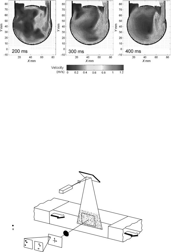
336 FLOWMETERS
Figure 15. Phase-average velocity maps from mid to late diastole for a prototype artificial heart ventricular chamber (time reference is from the onset of diastole, 4.7 L min 1 CO, 75 bpm) (68).
laser such that the camera shutter is centered between the firing of the two lasers. This synchronization technique is called frame straddling and produces two sequential images of each laser beam pulse. Although the time between successive camera frames may be much larger than the time duration between laser pulses, the two images of the particle field created are separated by the specified time interval between the two laser pulses.
A discussion of PIV must begin with a brief introduction of the terminology commonly used. Figure 17 provides a schematic representation of geometric imaging (66). The ‘‘light plane’’ is the ‘‘volume’’ of the fluid illuminated by the light sheet. The ‘‘image plane’’ is the image from the light plane captured on the CCD sensor. It is important to note that the light plane is a 3D space or volume, whereas the image plane is a 2D space or ‘‘surface.’’ The subvolume
selected from the light plane for cross correlation is called the interrogation subvolume. The corresponding location of this interrogation volume captured on the image plane is called the interrogation subregion. Please note that the displacement vectors in an interrogation volume are threecomponent vectors, whereas those in an interrogation area are two-component vectors. ‘‘Particle’’ is the physical particle suspended in the fluid volume. ‘‘Particle image’’ is the image of each particle in the image plane. Particle density, intensity, and pair refer to particle properties, whereas image density, intensity, and pair refer to particle image properties.
Most commercial systems use a cross-correlation-based image processing technique to compute the particle displacement. Images are subdivided into small interrogation regions, typically a fraction of the overall image size, and
Light sheet optics |
Mirror |
|
Laser |
|
|
|
|
Light sheet |
|
|
Illuminated |
Flow with |
|
particles |
tracer particles |
|
|
First light pulse at t |
|
|
Second light pulse at t′ |
|
|
y |
Imaging optics |
Flow direction |
x |
|
|
t′ |
Image plane |
|
t |
||
|
Figure 16. Schematic of a PIV setup (66). (With kind permission of Springer Science and Business Media.)
|
|
Interrogation |
|
|
Y |
volume |
|
|
|
||
|
|
X |
|
|
Z |
|
|
x |
z |
|
|
y |
|
Z0 |
|
|
|
||
Image |
Z0 |
Light sheet(S) |
|
plane |
Imaging |
||
(Thickness ∆ Z0 ) |
|||
|
lens |
Interrogation
area
Figure 17. Schematic representation of geometric imaging (66). (With kind permission of Springer Science and Business Media.)
the same two subregions are cross-correlated between the two images to obtain the average displacement of the particles within that subregion. From this displacement and the known time delay, the velocities within the interrogation region are obtained.
Statistical PIV assumes all particles in an interrogation subregion move a similar distance and direction. The processing algorithm then computes the mean displacement vector for the particles in the interrogation volume. Therefore, the local particle distribution pattern captured on each exposure should be similar; but the group of local particles is displaced from image to image. Statistical PIV is then ‘‘pattern recognition’’ of the particle distribution within an interrogation subregion, instead of the averaged
FLOWMETERS 337
particle displacements. Sophisticated pattern recognition schemes have been developed by a number of researchers; however, the cross-correlation tends to be the algorithm of choice. The use of a cross-correlation as opposed to an autocorrelation eliminates directional ambiguity in the velocity measurement. Most commercial systems use advanced cross-correlation algorithms, such as the HartCorrelation, developed to improve signal to noise in the correlation estimate and enhance resolution (70,71).
The cross-correlation function for two interrogation subregions of frames A and B is defined by:
RIIðs; G; DÞ ¼ hIðx; GÞI0ðx þ s; G0; DÞi |
(18) |
where s is the shifting vector of the second interrogation window, G is the series of location vectors for each particle in the interrogation volume, D is the displacement vector for each particle, x is the spatial domain vectors within the interrogation area, I is the intensity matrix for the interrogation area from frame A, and I’ is the intensity matrix for the interrogation area from frame B. A detailed mathematical derivation of the cross-correlation for (group) particle tracking is beyond the scope of this presentation. The location of the maximum value of cross-correlation function represents the mean particle displacement for the interrogation image. Figure 18 is an example of a cross-correlation function between two images.
The location of the cross-correlation peak should be determined with subpixel accuracy. Several curve-fitting algorithms have been developed to identify the peak in the cross-correlation. Gaussian, parabolic, and centroid are three commonly used methods in commercial software, although others exist. A Gaussian peak fit is most commonly used because the cross-correlation function of two Gaussian functions also yields a Gaussian function, which
Figure 18. Representative cross-correlation map between frames A and B.
338 FLOWMETERS
means that if the intensities of individual particle images in the interrogation area fit a Gaussian shape, the crosscorrelation function can be accurately approximated by the Gaussian function, which occurs only under the condition of low displacement gradient, so that the particle distribution pattern is preserved in windows A and B. The crosscorrelation function in distorted, particle image intensity distribution patterns are less accurately approximated by a Gaussian distribution. A three-point estimator for Gaussian fit works better with a narrow and symmetric peak. Centroid peak finding should be considered when the cross-correlation peak is expected to have asymmetric and irregular patterns. Such cases occur for particle images larger than 2–3 pixels in diameter, for a low intensity ratio of particle image to background noise, or for a high gradient displacement field. For ‘‘correlation-based correction,’’ the centroid peak finding might be more suitable than Gaussian because the multiplications could distort the cross-correlation peak.
The use of a digital CCD camera presents an error source known as ‘‘peak locking.’’ This error impacts the accuracy of the subpixel estimation in the correlation peak and thus impacts the velocity measurement. This error will be discussed later.
Like LDV and Doppler, PIV and PTV require that the fluid be seeded with tracer particles that follow the fluid motion. The particle density, the number of particles per unit volume of fluid, determines what technique should be used, PIV or PTV. Flows with a low particle density are more suited to PTV, wheras PIV works best in high particle density flows. It is assumed that the tracer particles follow the flow accurately to give an exact representation of the flow field at various times and locations. The particle density, however, should be sufficiently low to preserve the original flow dynamics. Such a dilute condition is expressed by the inequality:
ðrppdp4yrÞ=ð18m dp3Þ < 1 |
(19) |
where dp and rp are the particle diameter and density, respectively, m is fluid viscosity, ur is the averaged particle velocity relative to neighboring particles, and dp is the average distance between particles.
Particles must be small enough to follow the fluid flow but large enough to be seen. The particle relaxation time, ts, should be small relative to the flow time scales.
ts ¼ dp2ðrp=18mÞ |
(20) |
In practice, ts is made small by using very small particles. The Stokes number for PIV experiments, StPIV, can be
defined as ts/tPIV, where tPIV is the small finite separation time between two observations (pulse separation time).
StPIV should be much less than 1 to assure negligible particle-fluid velocity differences over the pulse separation. However, particles must be large enough to scatter sufficient light energy to be visualized on the recording device (e.g., a CCD camera) with the goal that a particle image is at least several pixels in size. Increasing the light source energy can improve visibility, but a saturation point is reached where increasing light source energy does not help. Furthermore, high energy can damage windows and plastic test models.
The time separation of the two laser pulses must be small enough to minimize particle loss through too large a particle displacement between the first and second frames of the interrogation window. However, the time separation must be long enough both to permit adequate displacement of particles at the lowest measurable velocities in each velocity component and to minimize the impact of pixel peak locking (72). Complex and highly 3D flows can be biased in a 2D PIV system. PIV can provide very high spatial resolution, but suffers from low temporal resolution. Furthermore, high magnification imaging used in high resolution PIV introduces additional constraints and limitations that must be overcome to achieve high quality vector maps.
The challenge for PIV is to correctly track particle motion. Figure 19 shows an example of a PIV particle image. The statistical cross-correlation approach is used to track the displacement of a ‘‘group’’ of particles within an indicated small volume or subregion. The location of a velocity vector is at the center of the subregion spot. The spatial resolution for a ‘‘velocity vector’’ in PIV is the size of the interrogation subregion. Overlapping adjacent interrogation subregions is commonly used to reduce the distance between adjacent vectors and provide additional vectors in the overall vector map. However, this overlapping does not increase the spatial resolution of the velocity field, which is limited to the size of the interrogation subregion.
Commercial PIV systems use a multigrid recursive method to reduce interrogation subregion size. In the hierarchical approach, a PIV measurement with large interrogation subregions is first computed. Subsequently, the initial interrogation area is evenly divided into smaller areas for processing. Each smaller interrogation area is offset by the displacement obtained from its parent interrogation area. This process is repeated until the smallest possible interrogation size is reached (e.g., 128 128 ! 64 64 ! 32 32 ! 16 16) for the given flow field. An iterative method can be applied at the final grid level.
Figure 19. Example of a PIV particle image.
Similar to the multigrid method, the iterative method uses the obtained displacement from the first cross correlation to offset the second window for the next cross correlation. The difference is that it does not break down the interrogation areas into smaller windows, which is repeated until the difference between the displacements from successive cross correlations is less than one pixel. If the window B is shifted by the converged displacement, windows A and B should be virtually the same, as long as the gradient is sufficiently low. Iterative cross correlation is another way to increase accuracy.
A minimum number of particle pairs (on the order of 10) are required in PIV processing. The particle density in the flow will determine the minimum size subregion that can be used to obtain adequate vector maps. Thus, the spatial resolution is governed by the particle density. Near solid surfaces, the particle density is often lower in flows with strong wall gradients. Reducing the interrogation window size increases spatial resolution. However, an overly small window causes in-plane particle loss due to particles moving out of the interrogation spot. Several techniques exist to capture the particles moving out of the window without enlarging the interrogation spot. The first is simply to enlarge the second window to cover the expected displaced particle. The original interrogation window (frame A) is enlarged to the same size as window B and zero-padded at the extended part. The second technique is to offset the second window to the location of anticipated displacement.
Errors in PIV processing can occur from several sources. The spatial resolution for a velocity vector is the dimension of the interrogation volume. If the particles are evenly distributed, the center of an interrogation volume can be used as the vector location. The accuracy of the ‘displacement depends on both the subpixel accuracy of the peak finding algorithm and the image quality. A one-tenth pixel is the most accurate (66). Time resolution for the velocity is the separation time between two pulses, as the information during this period is not recorded. The velocity error is composed of systematic and residual error. Systematic errors come from the algorithm and experiment setting or image quality, which can be minimized and uncertainty in the time separation. Residual errors are inherent in the processing, such as errors due to the peak finding algorithm. The residual errors are usually not a function of Dt. Therefore, a too small separation time increases the velocity error as this error is proportional to 1/Dt.
The following discussion is relevant to the effect of image quality on PIV accuracy. Large particle images can result in wide cross-correlation peaks, which can reduce the accuracy of the peak finding algorithm. In addition, large particles require larger interrogation spots to contain an appropriate number of particles, which leads to a reduction in spatial resolution. Particle images smaller than 2 pixels in diameter, or particle displacements that are less than 2 pixels, can introduce a displacement bias, called ‘‘peak locking.’’ The displacement peaks tend to be biased toward integer values. Peak locking presents itself as a ‘‘staircased’’ velocity pattern, in a region with a velocity gradient where the velocity distribution should be smooth. The calculation of spatial derivatives of this vector map then produces a mosaic pattern in the gradient map.
FLOWMETERS 339
Figure 20 illustrates these patterns. Techniques, such as multigrid or continuous window-shifting or iterative image deformation, have been proposed to overcome peak locking. Image preconditioning, such as filtering, or defocusing can optimize the image diameter. The resolution of the CCD sensor, therefore, also limits the use of smaller particles to increase the velocity resolution.
The methods developed to increase displacement accuracy rely on the assumption of low displacement gradient. High gradient tends to bias the displacement toward low values because the particles with smaller displacements are more likely to remain in the interrogation volume longer than those with higher displacements. This bias can be minimized by reducing the size of the interrogation volume and separation time. For high distortion of the particle pattern in a high gradient spot, the centroid peak finding algorithm is more suitable than the Gaussian. However, PTV, as it follows an individual particle, is not affected by high gradient. Several research groups use the displacement results from PIV to guide the local search areas for PTV in a coupled PIV/PTV processing algorithm. These coupled techniques relieve the gradient limit in PIV and increases resolution of both velocity vectors and velocity fields.
The motion across the light sheet in highly 3D flows can bias the local velocity estimation due to perspective projection, if the particle has not left the light sheet. The effect of perspective projection velocity bias, illustrated in Fig. 21 (68), is usually more severe at the edges of the image, where the projection angle increases. At high image magnification, the focal length becomes shorter and the projection angle increases, which worsens the perspective projection. Strong perspective projection could vary the magnification factor through the image plane resulting in an image distortion.
In general, the light sheet thickness is smaller than the depth of focus, dz. The light sheet thickness, therefore, determines the thickness of the effective interrogation volume: All illuminated particles are well focused. Most commercial systems using standard-grade Yag lasers with appropriate optics can generate light sheets that have a thickness on the order of 100–200 mm, although light sheets can be as thick as a 1 mm. In high magnification imaging, the depth of focus can become smaller than the light sheet thickness. The thickness of the effective interrogation volume is then constrained to the depth of focus. In this case, particles located beyond the focal plane but within the illuminated plane are out-of-focus and appear as highly nonuniform background image noise and can affect the cross correlation. In addition, the thickness of the effective interrogation volume determines the tolerance to out-of-plane motion. A smaller effective volume thickness increases the probability for out-of-plane particle loss. In general, the estimated maximum out-of-plane motion should be less than one-fourth of the effective volume thickness.
Data validation is another source of uncertainty in PIV. Bad velocity vectors will ultimately appear within a vector map due to noise in the displacement estimation. Several filtering algorithms have been developed to remove these bad vectors. These filter routines operate on thresholding velocity at a particular location and use either the
340 FLOWMETERS
Figure 20. (a) Staircased pattern in a velocity profile at a wall. (b) Gradient field calculation (bottom image) of a measured velocity field (top image) showing mosaic pattern (68).
magnitude of the velocity estimate, the mean, the median or the rms within a predefined subregion, or other more complicated thresholds to low pass filter the estimates. Improper application of a validation scheme can overfilter
Figure 21. Illustration of the perspective projection; the red arrow is the vector obtained from perspective projection, the blue is the correct projection of displacement vector on the XY plane (68).
the velocity map and throw away good data. For example, rms validation techniques should be carefully used in turbulent shear layers where high rms values are normally encountered. It is possible to inadvertently filter good instantaneous turbulent velocity ensembles with a tight rms filter setting. In general, some knowledge of the flow under study is needed to accurately perform vector validation.
Commercial PIV systems can be two-component or three-component, planar or volume systems. A twocomponent, planar PIV system provides information on two components of the velocity vector. In two-component PIV, the measured displacement vector is the projection of the three-component velocity vector on the 2D plane of the light sheet. Flow information for highly three-component flows can be inaccurately represented by planar PIV images. Stereographic and holographic PIV systems have been developed for three-component measurement in a plane or volume, respectively. Although the instantaneous velocity field obtained by PIV has an advantage over LDV (or Doppler), two-exposure PIV only provides information on the particle motion during the two exposures and also suffers from poor temporal frequency response in the measurement of adjacent vector maps in time. Particle acceleration cannot be measured by direct two-exposure PIV. Four-exposure systems have been developed to permit calculation of the particle acceleration by Hassan and Phillip (73) and Lui and Katz (74), although the temporal resolution for the acceleration is not yet comparable with that of LDV.
BIBLIOGRAPHY
Cited References
1.Fung YC. Respiratory gas flow. In: Biomechanics: Motion, Flow, Stress and Growth. New York: Springer-Verlag; 1990.
2.Primiano FP. ‘‘Measurements of the respiratory system. In: Webster JG, editor. Medical Instrumentation: Application and Design. New York: John Wiley & Sons; 1998.
3.Hampers CL, Schuback E, Lowrie EG, Lazarus JM. Clinical engineering in hemodialysis and anatomy of an artificial kidney unit. In: Long Term Hemodialysis. New York: Grune and Stratten; 1973.
4.Neuman MR. Therapeutic and prosthetic devices. In: Webster JG, ed., Medical Instrumentation: Application and Design. 3rd ed. New York: John Wiley & Sons; 1998.
5.Tedgui A, Lever MJ. Filtration through damaged and undamaged rabbit thoracic aorta. Am J Physiol 1984;247:784.
6.Jin S, Oshinski J, Giddens DP. Effects of wall motion and compliance on flow patterns in the ascending aorta. J Biomech Eng 2003;125:347–354.
7.Hochareon P, Manning KB, Fontaine AA, Tarbell JM, Deutsch S. Wall shear-rate estimation within the 50cc Penn State artificial heart using particle image velocimetry. J Biomech Eng 2004;126:430–437.
8.Hochareon P, Manning KB, Fontaine AA, Tarbell JM, Deutsch S. Correlation of in vivo clot deposition with the flow characteristics in the 50cc Penn State artificial heart: A preliminary study J ASAIO 2004;50(6):537–542.
9.Merzkirch W. Flow Visualization. New York: Academic Press; 1974.
10.Rouse H, Ince S. History of hydraulics. Iowa Institute of Hydraulics Research Report. Ames, (IA); State University of Iowa; 1957.
11.Latto B, El Riedy O, Vlachopoulos J. Effect of sampling rate on concentration measurements in nonhomogeneous dilute polymer solution flow. J Rheol 1981;25:583–590.
12.Lauchle GC, Billet ML, Deutsch S. Hydrodynamic measurements in high speed liquid flow facilities. Gad-el-Hak M. In: Lecture Notes in Engineering, 46, Experimental Fluid Mechanics. New York: Springer Verlag, 1989.
13.White KC, Kavanaugh JF, Wang DM, Tarbell JM. Hemodynamics and wall shear rate in the abdominal aorta of dogs. Circ Res 1994;75(4):637–649.
14.Povey MJW. Ultrasonic Techniques for Fluids Characterization. New York: Academic Press; 1997.
15.Siedband MP. Medical imaging systems. In: Webster J, editor. Medical Instrumentation: Application and Design. New York: John Wiley & Sons; 1998.
16.Adrian RJ. Particle imaging techniques for experimental fluid mechanics. Ann Rev Fluid Mech 1991;23:261–304.
17.Webster JG. Measurement of flow and volume of blood. In: Webster JG, editor. Medical Instrumentation: Application and Design. 3rd ed. New York: John Wiley & Sons; 1998.
18.Lipowski HH, McKay CB, Seki J. Transit time distributions of blood flow in the microcirculation. In: Lee, Skalak, editors. Microvascular Mechanics. New York: Springer Verlag; 1989. p 13–27.
19.Shaughnessy EJ, Katz IM, Schaffer JP. Introduction to Fluid Mechanics. New York: Oxford University Press; 2005.
20.Bendat JS, Peirsol AG. Random Data: Analysis and Measurement Procedures. New York: John Wiley and Sons; 1986.
21.Coleman HW, Steele WG. Experimentation and Uncertainty Analysis for Engineers. New York: John Wiley and Sons; 1999.
22.Montgomery DC. Design and Analysis of Experiments, 3rd ed. New York: John Wiley and Sons; 1991.
23.White FM. Fluid Mechanics. New York: McGraw-Hill; 1979.
FLOWMETERS 341
24.Caro CG, Pedley TJ, Schroter RC and Seed WA. The Mechanics of the Circulation. New York: Oxford University Press; 1978.
25.Pedley TJ, Schroter RC, Sudlow MF. Flow and pressure drop in systems of repeatedly branching tubes. J Fluid Mech 1971; 46(2):365–383.
26.Mori Y, Nakayama W. Study on forced convective heat transfer in curved pipes. Int J Heat Mass Transfer 1965;8:67–82.
27.Drost CJ. Vessel diameter-independent volume flow measurements using ultrasound. Proceedings of the San Diego Biomedical Symposium, 17, 1978: p 299–302.
28.Lynnworth LC. Ultrasonic flow meters. In: Mason WP, Thurston RN eds. Physical Acoustics. Academic Press; 1979.
29.Beldi G, Bosshard A, Hess OM, Althaus U and Walpoth BH. Transit time flow measurement: Experimental validation and comparison of three different systems. Ann Thorac Surg 2000;70:212–217.
30.Weyman AE. Principles and Practice of Echocardiography, 2nd ed., New York: Lea & Febiger; 1994.
31.Crowe CT, Sommerfeld M, Tsuji Y. Multiphase Flows with Droplets and Particles. Boca Raton (FL): CRC Press; 1998.
32.Comte-Bellot G. Hot-wire anemometry. Ann Rev Fluid Mech 1976;8:209–232.
33.Nerem RM, Rumberger JA, Gross DR, Muir WW, Geiger GL. Hot film coronary artery velocity measurements in horses. Cardiovasc Res 1976;10(3):301–313.
34.Nerem RM, Rumberger JA, Gross DR, Hamlin RL, Geiger GL. Hot film anemometer velocity measurements of arterial blood flow in horses. Circ Res 1974;34(2):193–203.
35.Falsetti HL, Carroll RJ, Swope RD, Chen CJ. Turbulent blood flow intheascendingaortaofdogs.CardiovascRes1983;17(7):427–436.
36.Baldwin, JT, Tarbell, JM, Deutsch S, Geselowitz DB, Rosenberg G, Hot-film wall shear probe measurements inside a ventricular assist device,’’ J Biomech Eng, 1988;110(4):326– 333.
37.Baldwin JT, Tarbell KM, Deutsch S, Geselowitz DB. Wall shear stress measurements in a ventricular assist device. J BioMech Eng 1988;V110:326–333.
38.BattenJR, NeremRM. Modelstudy offlowincurved and planar arterial bifurcations. Cardiovasc Res 1982;16(4):178–186.
39.Bruun HH. Hot Wire Anemometry: Principles and Signal Analysis. New York: Oxford University Press; 1995.
40.Stock DE Ed. Thermal anemometry 1993. Proceedings of the 3rd Int. Symposium on Thermal Anemometry – ASME Fluids Engineering Conference, Washington, (DC), FED 167 1993.
41.Otto, CM, The Practice of Clinical Echocardiography, Philadelphia, PA., WB Saunders Co., 1997.
42.Cape EG, Nanda NC, Yoganathan AP. Quantification of regurgitant flow through Bileaflet heart valves: theoretical and in vitro studies. Ultrasound Med Biol 1993;19:461–468.
43.Pettigrew RI. Magnetic resonance in cardiovascular imaging. In Zaret BL et al., editors. Frontiers in Cardiovascular Imaging. Baltimoc, MD: Raven Press; 1993.
44.Ku DN, Biancheri CL, Pettigrew RI, et al. Evaluation of magnetic resonance velocimetry for steady flow. J Biomech Eng 1990;112:464–472.
45.Hahn EL. Detection of sea-water motion by nuclear preemission. J Geophys Res 1960;65:776–777.
46.Singer JR, Crooks LE. Nuclear magnetic resonance blood flow measurements in the human brain. Science 1983;221:654–656.
47.Moran PR, Moran RA, Karstaedt N. ‘‘Verification and evaluation of internal flow and motion. True magnetic resonance imaging by the phase gradient modulation method.’’ Radiology. 1985 Feb; 154(2):433–41.
48.Bryant DJ, Payne JA, Firmin DN, Longmore DB. Measurement of flow with NMR imaging using a gradient pulse and phase difference technique. J Comp Assist Tomogr 1984;8: 588– 593.