

- •VOLUME 3
- •CONTRIBUTOR LIST
- •PREFACE
- •LIST OF ARTICLES
- •ABBREVIATIONS AND ACRONYMS
- •CONVERSION FACTORS AND UNIT SYMBOLS
- •EDUCATION, COMPUTERS IN.
- •ELECTROANALGESIA, SYSTEMIC
- •ELECTROCARDIOGRAPHY, COMPUTERS IN
- •ELECTROCONVULSIVE THERAPHY
- •ELECTRODES.
- •ELECTROENCEPHALOGRAPHY
- •ELECTROGASTROGRAM
- •ELECTROMAGNETIC FLOWMETER.
- •ELECTROMYOGRAPHY
- •ELECTRON MICROSCOPY.
- •ELECTRONEUROGRAPHY
- •ELECTROPHORESIS
- •ELECTROPHYSIOLOGY
- •ELECTRORETINOGRAPHY
- •ELECTROSHOCK THERAPY.
- •ELECTROSTIMULATION OF SPINAL CORD.
- •ELECTROSURGICAL UNIT (ESU)
- •EMERGENCY MEDICAL CARE.
- •ENDOSCOPES
- •ENGINEERED TISSUE
- •ENVIRONMENTAL CONTROL
- •EQUIPMENT ACQUISITION
- •EQUIPMENT MAINTENANCE, BIOMEDICAL
- •ERGONOMICS.
- •ESOPHAGEAL MANOMETRY
- •EVENT-RELATED POTENTIALS.
- •EVOKED POTENTIALS
- •EXERCISE FITNESS, BIOMECHANICS OF.
- •EXERCISE, THERAPEUTIC.
- •EXERCISE STRESS TESTING
- •EYE MOVEMENT, MEASUREMENT TECHNIQUES FOR
- •FETAL MONITORING
- •FETAL SURGERY.
- •FEVER THERAPY.
- •FIBER OPTICS IN MEDICINE
- •FICK TECHNIQUE.
- •FITNESS TECHNOLOGY.
- •FIXATION OF ORTHOPEDIC PROSTHESES.
- •FLAME ATOMIC EMISSON SPECTROMETRY AND ATOMIC ABSORPTION SPECTROMETRY
- •FLAME PHOTOMETRY.
- •FLOWMETERS
- •FLOWMETERS, RESPIRATORY.
- •FLUORESCENCE MEASUREMENTS
- •FLUORESCENCE MICROSCOPY.
- •FLUORESCENCE SPECTROSCOPY.
- •FLUORIMETRY.
- •FRACTURE, ELECTRICAL TREATMENT OF.
- •FUNCTIONAL ELECTRICAL STIMULATION
- •GAMMA CAMERA.
- •GAMMA KNIFE
- •GAS AND VACUUM SYSTEMS, CENTRALLY PIPED MEDICAL
- •GAS EXCHANGE.
- •GASTROINTESTINAL HEMORRHAGE
- •GEL FILTRATION CHROMATOGRAPHY.
- •GLUCOSE SENSORS
- •HBO THERAPY.
- •HEARING IMPAIRMENT.
- •HEART RATE, FETAL, MONITORING OF.
- •HEART VALVE PROSTHESES
- •HEART VALVE PROSTHESES, IN VITRO FLOW DYNAMICS OF
- •HEART VALVES, PROSTHETIC
- •HEART VIBRATION.
- •HEART, ARTIFICIAL
- •HEART–LUNG MACHINES
- •HEAT AND COLD, THERAPEUTIC
- •HEAVY ION RADIOTHERAPY.
- •HEMODYNAMICS
- •HEMODYNAMIC MONITORING.
- •HIGH FREQUENCY VENTILATION
- •HIP JOINTS, ARTIFICIAL
- •HIP REPLACEMENT, TOTAL.
- •HOLTER MONITORING.
- •HOME HEALTH CARE DEVICES
- •HOSPITAL SAFETY PROGRAM.
- •HUMAN FACTORS IN MEDICAL DEVICES
- •HUMAN SPINE, BIOMECHANICS OF
EVOKED POTENTIALS |
233 |
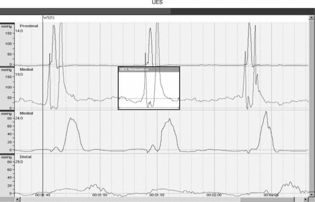
Figure 5. Manometric tracings of the upper esophageal sphincter. (Courtesy of Medtronic Corp., Minneapolis, MN.)
and Chagas’ disease. Nonspecific esophageal motility disorders are those that are associated with the patient’s symptoms, but the pattern of manometric dysmotility does not fit into the primary or secondary categories. Another category that is becoming better recognized and characterized is ineffective esophageal motility, which occurs when esophageal motility appears normal, but does not result in effective propagation of the food bolus down the esophagus.
BIBLIOGRAPHY
Cited References
1.Castell DO et al. Esophageal Motility Testing, 2nd ed. New York: Elsevier; 1993.
2.Castell JD, Dalton CB. Esophageal manometry. In: Castell DO, editor. The Esophagus. Boston:Little, Brown and Co.; 1992.
3.Stein HJ, Demeester TR, Hinder RA. Outpatient physiologic testing and surgical management of foregut motility disorders. Curr Prob Surg 1992;29:415–555.
See also ENDOSCOPES; GASTROINTESTINAL HEMORRHAGE.
ESU. See ELECTROSURGICAL UNIT (ESU).
EVENT-RELATED POTENTIALS. See EVOKED
POTENTIALS.
EVOKED POTENTIALS
RODRIGO QUIAN QUIROGA
University of Leicester
Leicester, United Kingdom
INTRODUCTION
Our knowledge about the brain has increased dramatically in the last decades due to the incorporation of new and extraordinary techniques. In particular, fast computers enable more realistic and complex simulations and boosted the emergence of computational neuroscience. With modern acquisition systems we can record simultaneously up to few hundred neurons and deal with issues like population coding and neural synchrony. Imaging techniques such as magnetic resonance imaging (MRI) allow an incredible visualization of the locus of different brain functions. On the other extreme of the spectrum, molecular neurobiology has been striking the field with extraordinary achievements. In contrast to the progress and excitement generated by these fields of neuroscience, electroencephalography (EEG) and evoked potentials (EPs) have clearly decreased in popularity. What can we learn from scalp electrodes recordings, when one can use sophisticated devices like MRI, or record from dozens of intracranial electrodes? Still a lot.
234 EVOKED POTENTIALS
There are mainly three advantages of the EEG: (1) it is relatively inexpensive; (2) it is noninvasive, and therefore it can be used in humans, (3) it has a very high temporal resolution, thus enabling the study of the dynamics of brain processes. These features make the EEG a very accessible and useful tool. It is particularly interesting for the analysis of high level brain processes that arise from the activity of large cell assemblies and may be poorly reflected by single neuron properties. Moreover, such processes can be well localized in time and even be reflected in time varying patterns (e.g., brain oscillations) that are faster than the time resolution of imaging techniques. The caveat of noninvasive EEGs is the fact that they reflect the average activity of sources far from the recording sites, and therefore do not have an optimal spatial resolution. Moreover, they are largely contaminated by noise and artifacts.
Although the way of recording EEG and EP signals did not change as much as multiunit recordings or imaging techniques, there have been significant advances in the methodology for analyzing the data. In fact, due to their high complexity, low signal/noise ratio, nonlinearity, and nonstationarity, they have been an ultimate challenge for most methods of signal analysis. The development and implementation of new algorithms that are specifically designed for such complex signals allow us to get information beyond the one accessible with previous approaches. These methods open a new gateway to the study of high level cognitive processes in humans with noninvasive techniques and at no great expense. Here, we review some of the most
common paradigms to elicit evoked potentials and describe basic and more advanced methods of analysis with special emphasis on the information that can be gained from their use. Although we focus on EEG recordings, these ideas also apply to magnetoencephalograpic (MEG) recordings.
RECORDING
The electroencephalogram measures the average electrical activity of the brain at different sites of the head. Typical recordings are done at the scalp with high conductance electrodes placed at specific locations according to the socalled 10–20 system (1). The activity of each electrode can be referenced to a common passive electrode (or to a pair of linked electrodes placed at the earlobes)—monopolar recordings—or can be recorded differentially between pairs of contiguous electrodes—bipolar recordings—. In the latter case, there are several ways of choosing the electrode pairs. Furthermore, there are specific montages of bipolar recordings designed to visualize the propagation of activity across different directions (1). Intracranial recordings are common in animal studies and are very rare in humans. Intracranial electrodes are mainly implanted in epileptic patients refractory to medication in order to localize the epileptic focus, and then evaluate the feasibility of a surgical resection.
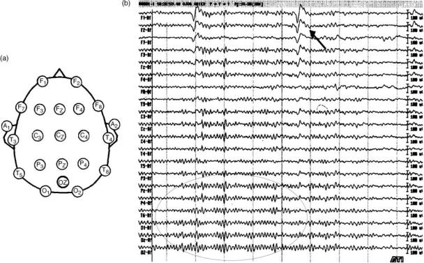
Figure 1 shows the 10–20 electrode distribution (a) and a typical monopolar recording of a normal subject with eyes
Figure 1. (a) Electrode montage of the 10–20 system and (b) an exemplary EEG recording with this montage. All electrodes are referenced to a linked earlobes reference (A1 and A2). F ¼ frontal, C ¼ central, P ¼ parietal, T ¼ temporal, and O ¼ occipital. Note the presence of blinking artifacts (marked with an arrow) and of posterior alpha oscillations (marked with an oval).
open (b). Note the high amplitude deflections in the anterior recordings due to blinking artifacts. In fact, one of the main problems in EEG analysis is the very low signal/noise ratio. Note also the presence of ongoing oscillations in the posterior sites. These oscillations are 10 Hz and are known as the alpha rhythm. The EEG brain oscillations of different frequencies and localizations have been correlated with functions, stages and pathologies of the brain (2–4).
In many scientific fields, especially in physics, one very useful way to learn about a system is by studying its reactions to perturbations. In brain research, it is also a common strategy to see how single neurons or large neuronal assemblies, as measured by the EEG, react to different types of stimuli. Evoked potentials are the changes in the ongoing EEG activity due to stimulation. They are time locked to the stimulus and they have a characteristic pattern of response that is more or less reproducible under similar experimental conditions. They are characterized by their polarity and latency, for example, P100 meaning a positive deflection (P for positive) occurring 100 ms after stimulation. The recording of evoked potentials is done in the same way as the EEGs. The stimulus delivery system sends triggers to identify the stimuli onsets and offsets.
GENERATION OF EVOKED POTENTIALS
Evoked potentials are usually considered as the timelocked and synchronized activity of a group of neurons that add to the background EEG. A different approach explains the evoked responses as a reorganization of the ongoing EEG (3,5). According to this view, evoked potentials can be generated by a selective and time-locked enhancement of a particular frequency band or by a phase resetting of ongoing frequencies. In particular, the study of the EPs in the frequency domain attracted the attention of several researchers (see section on Event-Related Oscillations). A few of these works focus on correlations between prestimulus EEG and the evoked responses (4).
SENSORY EVOKED POTENTIALS
There are mainly three modalities of stimulation: visual, auditory, and somatosensory. Visual evoked potentials are usually evoked by light flashes or visual patterns such as a checkerboard or a patch. Figure 2 shows the grand average visual evoked potentials of 10 subjects. Scalp electrodes were placed according to the 10–20 system, with linked earlobes reference. The stimuli were a color reversal of the (black/white) checks in a checkerboard pattern (sidelength of the checks: 50’). There is a positive deflection at 100 ms after stimulus presentation (P100) followed by a negative rebound at 200 ms (N200). These peaks are best defined at the occipital electrodes, which are the closest to the primary visual area. The P100 is also observed in the central and frontal electrodes, but not as well defined and appearing later than in the posterior sites. The P100–N200 complex can be seen as part of an 10 Hz event-related oscillation as it will be described in the following sections. Visual EPs can be used clinically to identify lesions in the
EVOKED POTENTIALS |
235 |
Figure 2. Grand average visual evoked potential. There is mainly one positive response at 100 ms after stimulation (P100) followed by a negative one at 200 ms (N200). These responses are best localized in the posterior electrodes.
visual pathway, such as the ones caused by optic neuritis and multiple sclerosis (6–9).
Auditory evoked potentials are usually elicited by tones or clicks. According to their latency they are further subdivided into early, middle, and late latency EPs. Early EPs comprise: (1) the electrococheleogram, which reflects responses in the first 2.5 ms from the cochlea and the auditory nerve, and (2) brain stem auditory evoked potentials (BSAEP), which reflect responses from the brain stem in the first 12 ms after stimulation and are recorded from the vertex. The BSAEP are seen at the scalp due to volume conduction. Early auditory EPs are mainly used clinically to study the integrity of the auditory pathway (10–12). They are also useful for detecting hearing impairments in children and in subjects that cannot cooperate in behavioral audiometry studies. Moreover, the presence of early auditory EPs may be a sign of recovery from coma.
Middle latency auditory EPs are a series of positive and negative waves occurring between 12 and 50 ms after stimulation. Clinical applications of these EPs are very limited due to the fact that the location of their sources is still controversial (10,11). Late auditory EPs occur between 50 and 250 ms after stimulation and consist of four main peaks labeled P50, N100, P150, and N200 according to their polarity and latency. They are of cortical origin and have a maximum amplitude at vertex locations. Auditory stimulation can also elicit potentials with latencies of > 200 ms. These are, however, responses to the context of the
236 EVOKED POTENTIALS
stimulus rather than to its physical characteristics and will be further described in the next section.
Somatosensory EPs are obtained by applying short lasting currents to sensory and motor peripheral nerves and are mainly used to identify lesions in the somatosensory pathway (13). In particular, they are used for the diagnosis of diseases affecting the white matter like multiple sclerosis, for noninvasive studies of spinal cord traumas and for peripheral nerve disorders (13). They are also used for monitoring the spinal cord during surgery, giving an early warning of a potential neurological damage in anesthetized patients (13).
Evoked potentials can be further classified as exogenous and endogenous. Exogenous EPs are elicited by the physical characteristics of the external stimulus, such as intensity, duration, frequency, and so on. In contrast, endogenous EPs are elicited by internal brain processes and respond to the significance of the stimulus. Endogenous EPs can be used to study cognitive processes as discussed in the next section.
EVOKED POTENTIALS AND COGNITION
Usually, the term evoked potentials refers to EEG responses to sensory stimulation. Sequences of stimuli can be organized in paradigms and subjects can be asked to perform different tasks. Event-related potentials (ERPs) constitute a broader category of responses that are elicited by ‘‘events’’, such as the recognition of a ‘‘target’’ stimulus or the lack of a stimulus in a sequence.
Oddball Paradigm and P300
The most common method to elicit ERPs is by using the oddball paradigm. Two different stimuli are distributed pseudorandomly in a sequence; one of them appearing frequently (standard stimulus), the other one being a target stimulus appearing less often and unexpectedly. Standard and target stimuli can be tones of different frequencies, figures of different colors, shapes, and so on. Subjects are usually asked to count the number of target appearances in a session, or to press a button whenever a target stimulus appears.
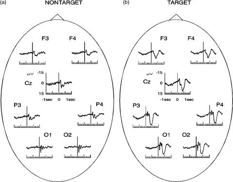
Figure 3 shows grand-average (10 subjects) visual evoked potentials elicited with an oddball paradigm. Figure 3 a shows the average responses to the frequent (non target) stimuli and (b) shows one to the targets. The experiment was the same as the one described in Fig. 2, but in this case target stimuli were pseudorandomly distributed within the frequent ones. Frequent stimuli (75%) were color reversals of the checks, as in the previous experiment, and target stimuli (25%) were also color reversals but with a small displacement of the checkerboard pattern (see Ref. (14) for details). Subjects had to pay attention to the appearance of the target stimuli.
The responses to the nontarget stimuli are qualitatively similar to the responses to visual EPs (without a task) shown in Fig. 2. As in the case of pattern visual EPs, the P100–N200 complex can be observed upon nontarget and target stimulation. These peaks are mainly related with primary sensory processing due to the fact that they do not depend on the task, they have a relatively short latency
Figure 3. Grand-average pattern visual evoked potentials with an oddball paradigm. (a) Average responses for the nontarget stimuli and (b) average responses for the target stimuli. Note the appearance of a positive deflection at 400 ms after stimulation (P300) only upon the target stimuli.
(100 ms) and they are best defined in the primary visual area (occipital lobe). Note, however, that these components can also modulate their amplitude in tasks with different attention loads (15,16). Target stimulation led to a marked positive component, the P300, occurring between 400 and 500 ms. The P300 is larger in the central and posterior locations.
While the localization of the P300 in the scalp is well known, the localization of the sources of the P300 in the brain are still controversial (for a review see Ref. (17). Since the P300 is task dependent and since it has a relatively long latency, it is traditionally related to cognitive processes such as signal matching, recognition, decision making, attention and memory updating (6,18,19). There have been many works using the P300 to study cognitive processes [for reviews see Refs. (18–20)]. In various pathologies cognition is impaired and this is reflected in abnormal P300 responses, as shown in depression, schizophrenia, dementia and others [for reviews see (18,21)].
The P300 can be also elicited by a passive oddball paradigm (i.e., an oddball sequence without any task). In this case, a P300 like response appears upon target stimulation, reflecting the novelty of the stimulus rather than the execution of a certain task. This response has been named P3a. It is earlier than the classic P300 (also named P3b), it is largest in frontal and central areas and it habituates quickly (22,23).
Mismatch Negativity
Mismatch negativity (MMN) is a negative potential elicited by auditory stimulation. It appears along with any change in some repetitive pattern and peaks between 100 and 200 ms after stimulation (24). It is generally elicited by the passive (i.e., no task) auditory oddball paradigm and it is visualized by subtracting the frequent stimuli from the deviant one. The MMN is generated in the auditory cortex. It is known to reflect auditory memory (i.e., the memory trace of preceding stimuli) and can be elicited even in the absence of attention (25). It provides an index of sound discrimination and has therefore being used to study dyslexia (25). Since MMN reflects a preattentive state, it can be also elicited during sleep (26). Moreover, it has been proposed as an index for coma prognosis (27,28).
Omitted Evoked Potentials
Omitted evoked potentials (OEPs) are similar in nature to the P300 and MMN, but they are evoked by the omission of a stimulus in a sequence (29–31). The nice feature of these potentials is that they are elicited without external stimulation, thus being purely endogenous components. Omitted evoked potentials mainly reflect expectancy (32) and are modulated by attention (31,33). The main problem in recording OEPs is the lack of a stimulus trigger. This results in large latency variations from trial to trial, and therefore OEPs may not be visible after ensemble averaging. Note that trained musicians were shown to have less variability in the latency of the OEP responses (latency jitter) in comparison to non-musicians due to their better time-accuracy (34).
EVOKED POTENTIALS |
237 |
Contingent Negative Variation
Contingent negative variation (CNV) is a slowly rising negative shift appearing before stimulus onset during periods of expectancy and response preparation (35). It is usually elicited by tasks resembling conditioned learning experiments. A first stimulus gives a preparatory signal for a motor response to be carried out at the time of a second stimulus. The CNV reflects the contingency or association between the two stimuli. It has been useful for the study of aging and different psychopathologies, such as depression and schizophrenia (for reviews see Refs. (36,37)). Similar in nature to the CNVs are the ‘‘Bereitschaft’’ or ‘‘Readiness’’ potentials (38), which are negative potential shifts preceeding voluntary movements [for a review see Ref. (36)].
N400
Of particular interest are ERPs showing signs of language processing. Kutas and Hillyard (39,40) described a negative deflection between 300 and 500 ms after stimulation (N400), correlated with the appearance of semantically anomalous words in otherwise meaningful sentences. It reflects ‘‘semantic memory’’; that is, the predictability of a word based on the semantic content of the preceding sentence (16).
Error Related Negativity
The error related negativity (ERN) is a negative component that appears after negative feedback (41,42). It can be elicited with a wide variety of reaction time tasks and it peaks within 100 ms of an error response. It reaches its maximum over frontal and central areas and convergent evidence from source localization analyses and imaging studies point toward a generation in the anterior cingulated cortex (41).
BASIC ANALYSIS
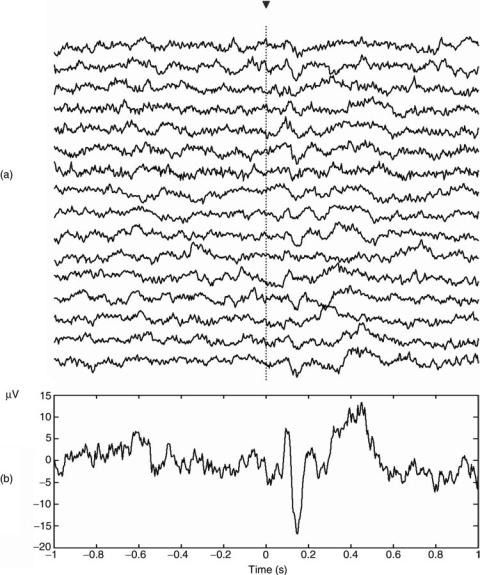
Figure 4a shows 16 single-trial visual ERPs from the left occipital electrode of a typical subject. These are responses to target stimuli using the oddball paradigm described in the previous section. Note that it is very difficult to distinguish the single-trial ERPs due to their low amplitude and due to their similarity to spontaneous fluctuations in the EEG. The usual way to improve the visualization of the ERPs is by averaging the responses of several trials. Since evoked potentials are locked to the stimulus onset, their contribution will add, whereas one of the ongoing EEG will cancel. Figure 4b shows the average evoked potential. Here it is possible to identify the P100, N200, and P300 responses described in the previous section.
The main quantification of the average ERPs is by means of their amplitudes and latencies. Most research using ERPs compare statistically the distribution of peak amplitudes and latencies of a certain group (e.g., subjects in some particular state or doing some task) with a matched control group. Such comparisons also can be used clinically and, in general, pathological cases show peaks with long latencies and small amplitudes (2,6).
238 EVOKED POTENTIALS
Figure 4. (a) Sixteen single-trial responses of a typical subject and
(b) the average response. The triangle marks the time of stimulation. Note that the evoked responses are clearly seen after averaging, but are hardly identified in the single trials.
Another important aspect of ERPs is their topography. In fact, the abnormal localization of evoked responses can have clinical relevance. The usual way to visualize the topography of the EPs is via contour plots (43–47). These are obtained from the interpolation of the EP amplitudes at fixed times. There are several issues to consider when analyzing topographic plots: (1) the way the 3D head is projected into two dimensions, (2) the choice of the reference, (3) the type of interpolation used, and (4) the number of electrodes and their separation (46). These choices can indeed bias the topographic maps obtained.
SOURCE LOCALIZATION
In the previous section, we briefly discussed the use of topographic representations of the EEG and EPs. Besides the merit of the topographic representation given by these maps, the final goal is to get a hint on the sources of the activity seen at the scalp. In other words, given a certain
distribution of voltages at the scalp one would like to estimate the location and magnitude of their sources of generation. This is known as the inverse problem and it has no unique solution. The generating sources are usually assumed to be dipoles, each one having six parameters to be estimated, three for its position and three for its magnitude. Clearly, the complexity of the calculation increases rapidly with the number of dipoles and, in practice, no more than two or three dipoles are considered. Dipole sources are usually estimated using spherical head models. These models consider the fact that the electromagnetic signal has to cross layers of different impedances, such as the dura mater and the scull. A drawback of spherical head models is the fact that different subjects have different head shapes. This led to the introduction of realistic head models, which are obtained by modeling the head shape using MRI scans and computer simulations. Besides all these issues, there are already some impressive results in the literature [see Refs. (49,86)] and references cited therein describing the use and applications of the LORETA

software; Ref. (50) and an extensive list of publications using the BESA software at http://www.besa.de). Since a reasonable estimation of the EEG and EP sources critically depends on the number of electrodes, dipole location has been quite popular for the analysis of magnetoencephalograms, which have more recording sites.
EVENT-RELATED OSCILLATIONS
Evoked responses appear as single peaks or as oscillations generated by the synchronous activation of a large network. The presence of oscillatory activity induced by different type of stimuli has been largely reported in animal studies. Bullock (51) gives an excellent review of the subject going from earlier studies by Adrian (52) to more recent results in the 1990s (some of the later studies are included in Ref. (53). Examples are event-related oscillations of 15– 25 Hz in the retina of fishes in response to flashes (54), gamma oscillations in the olfactory bulb of cats and rabbits after odor presentation (55,56) and beta oscillations in the olfactory system of insects (57,58). Moreover, it has been proposed that these brain oscillations play a role in information processing (55). This idea became very popular after the report of gamma activity correlated to the binding of perceptual information in anesthetized cats (59).
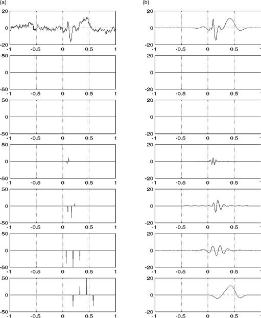
Event-related oscillations in animals are quite robust and in many cases visible by the naked eye. In humans, this activity is more noisy and localized in time. Consequently, more sophisticated time–frequency representations, like the one given by the wavelet transform, are needed in order to precisely localize event-related oscillations both in time and frequency. We finish this section with a cautionary note about event-related oscillations, particularly important for human studies. Since oscillations are usually not clear in the raw data, digital filters are used in order to visualize them. However, one should be aware that digital filters can introduce ‘‘ringing effects’’ and single peaks in the original signal can look like oscillations after filtering. In Fig. 5, we exemplify this effect by showing a delta function (a) filtered with a broad and a narrow band elliptic filter (b,c, respectively). Note that the original delta function can be mistaken for an oscillation after filtering, especially with the narrow band filter [see also Ref. (51)].
WAVELET TRANSFORM AND EVENT-RELATED OSCILLATIONS
Signals are usually represented either in the time or in the frequency domain. The best time representation is given by the signal itself and the best frequency representation is given by its Fourier transform (FT). With the FT it is possible to estimate the power spectrum of the signal, which quantifies the amount of activity for each frequency. The power spectrum has been the most successful method for the analysis of EEGs (2), but it lacks time resolution. Since event-related oscillations appear in a short time range, a simultaneous representation in time and frequency is more appropriate.
The Wavelet transform (WT) gives a time–frequency representation that has two main advantages: (1) optimal
EVOKED POTENTIALS |
239 |
Figure 5. A delta function (a) after broad (b) and narrow (c) band pass filtering. Note that single peaks can look like oscillations due to filtering.
resolution in the time and frequency domains; (2) no requirement of stationarity. It is defined as the correlation between the signal x(t) and the wavelet functions ca;bðtÞ
Wc Xða; bÞ ¼ hxðtÞjca;bðtÞi |
ð1Þ |
where ca;bðtÞ are dilated (contracted) and shifted versions of a unique wavelet function c(t)
ca;b ¼ jaj 1=2c t b ð2Þ a
(a, b are the scale and translation parameters, respectively). The WT gives a decomposition of x(t) in different scales, tending to be maximum at those scales and time locations where the wavelet best resembles x(t). Moreover, Eq. 1 can be inverted, thus giving the reconstruction of x(t).
The WT maps a signal of one independent variable t onto a function of two independent variables a, b. This procedure is redundant and not efficient for algorithm implementations. In consequence, it is more practical to define the WT only at discrete scales a and discrete times b by choosing the set of parameters fa j ¼ 2 j; b j; k ¼ 2 jkg, with integers j, k.
Contracted versions of the wavelet function match the high frequency components of the original signal and the dilated versions match low frequency oscillations. Then, by correlating the original signal with wavelet functions of different sizes we can obtain the details of the signal at different scales. The correlations with the different wavelet functions can be arranged in a hierarchical scheme called multiresolution decomposition (60). The multiresolution decomposition separates the signal into ‘‘details’’ at different scales and the remaining part is a coarser representation named ‘‘approximation’’.
Figure 6 shows the multiresolution decomposition of the average ERP shown in Fig. 4. The left part of the figure shows the wavelet coefficients and the right part shows the corresponding reconstructed waveforms. After a five octave wavelet decomposition using B-Spline wavelets (see Refs. 14,61 for details) the coefficients in the following bands were obtained (in brackets the EEG frequency bands that approximately correspond to these values): D1: 63– 125 Hz, D2: 31–62 Hz (gamma), D3: 16–30 Hz (beta), D4:

240 EVOKED POTENTIALS
Figure 6. Multiresolution decomposition (a) and reconstruction
(b) of an average evoked potential. D1–D5 and A5 are the different scales in which the signal is decomposed.
8–15 Hz (alpha), D5: 4–7 Hz (theta), and A5: 0.5–4 Hz (delta). Note that the addition of the reconstructed waveforms of all frequency bands returns the original signal. In the first 0.5 s after stimulation there is an increase in the alpha and theta bands (D4, D5) correlated with P100–N200 complex and later there is an increase in the delta band (A5) correlated with the P300. As an example of the use of wavelets for the analysis of event related oscillations, in the following we focus on the responses in the alpha band.
The grand average (across subjects) ERP is shown on left side of Fig. 7. Upper plots correspond to the responses to NT stimuli and lower plots to T stimuli. Only left electrodes and Cz are shown, the responses of the right electrodes being qualitatively similar. For both stimulus types we observe the P100–N200 complex and the P300 appears only upon target stimulation. Center and right plots of Fig. 7 show the alpha band wavelet coefficients and the filtered ERPs reconstructed from these coefficients, respectively. Amplitude increases are distributed over the entire scalp for the two stimulus types, best defined in the occipital electrodes. They appear first in the occipital electrodes, with an increasing delay in the parietal, cen-
tral, and frontal locations. The fact that alpha responses are not modulated by the task and the fact that their maximal and earliest appearance is in occipital locations (the primary visual sensory area) point toward a distributed generation and a correlation with sensory processing (14,61). Note that these responses are localized in time, thus stressing the use of wavelets.
In recent years, there have been an increasing number of works applying the WT to the study of event-related oscillations. Several of these studies dealt with gamma oscillations, encouraged by the first results by Gray and coworkers (59). In particular, induced gamma activity has been correlated to face perception (62), coherent visual perception (63), visual search tasks (64) cross-modal integration (64,65), and so on.
Another interesting approach to study event-related oscillations is the one given by the concepts of event-related synchronization (ERS) and event-related desynchronization (ERD), which characterize increases and decreases of the power in a given frequency band (66,67). Briefly, the band limited power is calculated for each single trial and then averaged across trials. Since ERS and ERD are defined as an
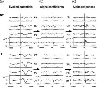
Figure 7. Grand average visual EPs to nontarget (NT) and target
(T) stimuli in an oddball paradigm (a). Both bþ and c plots shows the wavelet coefficients in the alpha band and the corresponding reconstruction of the signal from them, respectively.
average of the power of the signal, they are sensitive to phase locked as well as nonphase locked oscillations. Interestingly, similar concepts and a simple measure of phase locking can be also defined using wavelets (68).
SINGLE–TRIAL ANALYSIS
As shown in Fig. 4, averaging several trials increases the signal/noise ratio of the EPs. However, it relies on the basic assumption that EPs are an invariant pattern perfectly locked to the stimulus that lays on an independent stationary and stochastic background EEG signal. This assumption is in a strict sense not valid. In fact, averaging implies a loss of information related to systematic or unsystematic variations between the single trials. Furthermore, these variations (e.g., latency jitters) can affect the validity of the average EP as a representation of the single trial responses.
Several techniques have been proposed to improve the visualization of the single-trial EPs. Some of these approaches involve the filtering of single-trial traces by using techniques that are based on the Wiener formalism. This provides an optimal filtering in the mean-square error sense (69,70). However, these approaches assume that the signal is a stationary process and, since the EPs are compositions of transient responses with different time and frequency localizations, they are not likely to give optimal results. A obvious advantage is to implement time-varying strategies. In the following, we describe a recently proposed denoising implementation based on the WT to obtain the EPs at the single trial level (71,72). Other works also reported the use of wavelets for filtering average EPs or for visualizing the EPs in the single trials (73–77) see a brief discussion of these methods in Ref. 72.
In Fig. 6, we already showed the wavelet decomposition and reconstruction of an average visual EP. Note that the
EVOKED POTENTIALS |
241 |
P100–N200 response is mainly correlated with the first poststimulus coefficient in the details D4–D5. The P300 is mainly correlated with the coefficients at 400–500 ms in A5. This correspondence is easily identified because: (1) the coefficients appear in the same time (and frequency) range as the EPs and (2) they are relatively larger than the rest due to phase-locking between trials (coefficients related with background oscillations are diminished in the average). A straightforward way to avoid the fluctuations related with the ongoing EEG is by equaling to zero those coefficients that are not correlated with the EPs. However, the choice of these coefficients should not be solely based on the average EP and it should also consider the time ranges in which the single-trial EPs are expected to occur (i.e., some neighbor coefficients should be included in order to allow for latency jitters).
Figure 8a shows the coefficients kept for the reconstruction of the P100–N200 and P300 responses. Figure 8b shows the contributions of each level obtained by eliminating all the other coefficients. Note that in the final reconstruction of the average response (uppermost right plot) background EEG oscillations are filtered. We should remark that this is usually difficult to be achieved with a Fourier filtering approach due to the different time and frequency localizations of the P100–N200 and P300 responses, and also due to the overlapping frequency components of these peaks and the ongoing EEG. In this context, the main advantage of Wavelet denoising over conventional filtering is that one can select different time windows for the different scales. Once the coefficients of interest are identified from the average ERP, we can apply the same procedure to each single trial, thus filtering the contribution of background EEG activity.
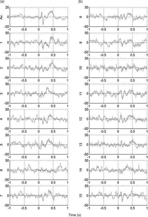
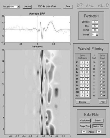
Figure 9 shows the first 15 single trials and the average ERP for the recording shown in the previous figure. The raw single trials have been already shown in Fig. 4. Note that with denoising (red curves) we can distinguish the P100–N200 and the P300 in most of the trials. Note also that these responses are not easily identified in the original signal (gray traces) due to their similarity with the ongoing EEG. We can also observe some variability between trials. For an easier visualization Fig. 10 shows a contour plot of the single trial ERPs after denoising. This figure is the output of a software package for denoising EPs (EP_den) available at www.vis.caltech.edu/ rodri. In the denoised plot, we observe a gray pattern followed by a black one between 100 and 200 ms, corresponding to the P100–N200 peaks. The more unstable and wider gray pattern at 400– 600 ms corresponds to the P300. In particular, it has been shown that wavelet denoising improves the visualization of the single trial EPs (and the estimation of their amplitudes and latencies) in comparison with the original data and in comparison with previous approaches, such as Wiener filtering (72).
APPLICATIONS OF SINGLE-TRIAL ANALYSIS
The single-trial analysis of EPs has a wide variety of applications. By using correlations between the average EP and the single-trial responses, it is possible to calculate
242 EVOKED POTENTIALS
Figure 8. Principle of wavelet denoising. The reconstruction of the signal is done using only those coefficients correlated with the EPs. See text for details.
selective averages including only trials with good responses (71,72). Moreover, it is possible to eliminate effects of latency jitters by aligning trials according to the latency of the single-trial peaks (71,72). The use of selective averages as well as jitter corrected averages had been proposed long ago (78,79). Wavelet denoising improves the identification of the single-trials responses, thus facilitating the construction of these averages.
Some of the most interesting features to study in singletrial EPs are the changes in amplitude and latency of the peaks from trial to trial. It is possible to calculate amplitude and latency jitters: information that is not avail-
able in the average EPs. For example, trained musicians showed smaller latency jitters of omitted evoked potentials in comparison with nonmusicians (34). Variations in amplitude and latency can be also systematic. Exponential decreases in different EP components have been related to habituation processes both in humans and in rats (80–82). Furthermore, the appearance of a P3-like component in the rat entorhinal cortex has been correlated to the learning of a go/no-go task (83). In humans, it has recently been shown that precise timing of the single-trial evoked responses accounts for a sleep-dependent automatization of perceptual learning (84).
EVOKED POTENTIALS |
243 |
Figure 9. Average EP and the single-trial responses corresponding to the data shown in the previous figure, with (black) and without (gray) denoising. Note that after denoising it is possible to identify the single-trial responses.
244 EVOKED POTENTIALS
Figure 10. Contour plot of the single-trial responses shown in the previous figure. The graphic user interface used to generate this plot is available at www.vis.caltech.edu/rodri.
CONCLUDING COMMENT
In addition to clinical applications, EPs are very useful to study high level cognitive processes. Their main advantages over other techniques are their low cost, their noninvasiveness and their good temporal resolution. Of particular interest is the study of trial-to-trial variations during recording sessions. Supported by the use of new and powerful methods of signal analysis, the study of single trial EPs and their correlation to different behavioral processes seems one of the most interesting directions of future research. In conclusion, the good and old EEG and its cousin, the EP, have a lot to offer, especially when new and powerful methods of analysis are applied.
BIBLIOGRAPHY
Cited References
1.Reilly EL. EEG recording and operation of the apparatus. In: Niedermeyer E, Lopes da Silva F, editors. Electroencephalography: Basic principles, clinical applications and related fields. Baltimore: Williams and Wilkins; 1993.
2.Niedermeyer E, Lopes da Silva F, editors. Electroencephalography: Basic principles, clinical applications and related fields. Baltimore: Williams and Wilkins; 1993, p 1097– 1123.
3.Bas¸ar E. EEG-Brain dynamics. Relation between EEG and brain evoked potentials. Amsterdam: Elsevier; 1980.
4.Bas¸ar E. Brain function and oscillations. Vol. I: Brain oscillations, principles and approaches. Vol. II: Integrative brain function: Neurophysiology and cognitive processes. Berlin- Heidelberg-New York: Springer; 1999.
5.Sayers B, Beagley HA, Hanshall WR. The mechanisms of auditory evoked EEG responses. Nature (London) 1974;247: 481–483.
6.Regan D. Human brain electrophysiology. Evoked potentials and evoked magnetic fields in science and medicine. Amsterdam: Elsevier; 1989.
7.Celesia GG. Visual evoked potentials and electroretinograms. In: Niedermeyer E, Lopes da Silva F, editors. Electroencephalography: Basic principles, clinical applications and related fields. Baltimore: Williams and Wilkins; 1993.
8.Desmetdt JE, editor. Visual evoked potentials in man: new developments. Oxford: Clarendon Press; 1977a.
9.Epstein CM. Visual evoked potentials. In: Daly DD, Pedley TA, editor. Current practice of clinical electroencephalography. New York: Raven Press; 1990.
10.Celesia GG, Grigg MM. Auditory evoked potentials. In: Niedermeyer E, Lopes da Silva F, editors. Electroencephalography: Basic principles, clinical applications and related fields. Baltimore: Williams and Wilkins; 1993.
11.Picton TW. Auditory evoked potentials. In: Daly DD, Pedley TA, editors. Current practice of clinical electroencephalography. New York: Raven Press; 1990.
12.Desmetdt JE, editor. Auditory evoked potentials in man. Basel: S. Karger; 1977b.
13.Erwin CW, Rozear MP, Radtke RA, Erwin AC. Somatosensory evoked potentials. In: Niedermeyer E, Lopes da Silva F, editors. Electroencephalography: Basic principles, clinical applications and related fields. Baltimore: Williams and Wilkins; 1993.
14.Quian Quiroga R, Schu¨ rmann M. Functions and sources of event-related EEG alpha oscillations studied with the Wavelet Transform. Clin Neurophysiol 1999;110:643–655.
15.Hillyard SA, Hink RF, Schwent VL, Picton TW. Electrical signs of selective attention in the human brain. Science 1973;182:177–179.
16.Hillyard SA, Kutas M. Electrophysiology of cognitive processing. Ann Rev Psychol 1983;34:33–61.
17.Molnar M. On the origin of the P3 event-related potential component. Int J Psychophysiol 1994;17:129–144.
18.Picton TW. The P300 wave of the human event-related potential. J Clin Neurophysiol 1992;9:456–479.
19.Polich J, Kok A. Cognitive and biological determinants of P300: an integrative review. Biol Psychol 1995;41:103–146.
20.Pritchard WS. Psychophysiology of P300. Psychol Bull 1984;89:506–540.
21.Polich J. P300 in clinical applications: Meaning, method and measurement. Am J EEG Technol 1991;31:201–231.
22.Polich J. Neuropsychology of P3a and P3b: A theoretical overvier. In: Arikan K, Moore N, editors. Advances in Electrophysiology in Clinical Practice and Research. Wheaton (IL): Kjellberg; 2002.
23.Polich J, Comerchero MD. P3a from visual stimuli: Typicality, task, and topography. Brain Topogr 2003;15:141–152.
24.Naatanen R, Tervaniemi M, Sussman E, Paavilainen P, Winkler I. ‘Primitive intelligence’ in the auditory cortex. Trends Neurosci 2001;24:283–288.
25.Naatanen R. Mismatch negativity: clinical research and possible applications. Int J Psychophysiol 2003;48:179–188.
26.Atienza M, Cantero JL. On-line processing of complex sounds during human REM sleep by recovering information from long-term memory as revealed by the mismatch negativity. Brain Res 2001;901:151–160.
27.Kane NM, Curry SH, Butler SR, Gummins BH. Electrophysiological indicator of awakening from coma. Lancet 1993; 341:688.
28.Fischer C, Morlet D, Bouchet P, Luante J, Jourdan C, Salford F. Mismatch negativity and late auditory evoked potentials in comatose patients. Clin Neurophysiol 1999;11:1601–1610.
29.Simson R, Vaughan HG Jr, Ritter W. The scalp topography of potentials associated with missing visual or auditory stimuli. Electr Clin Neurophysiol 1976;40:33–42.
30.Ruchkin DS, Sutton S, Munson R, Silver K, Macar F. P300 and feedback provided by absence of the stimulus. Psychophysiology 1981;18:271–282.
31.Bullock TH, Karamursel S, Achimowics JZ, McClune MC, Basar-Eroglu C. Dynamic properties of human visual evoked and omitted stimulus potentials. Electr Clin Neurophysiol 1994;91:42–53.
32.Jongsma MLA, Eichele T, Quian Quiroga R, Jenks KM, Desain P, Honing H, VanRijn CM. The effect of expectancy on omission evoked potentials (OEPs) in musicians and nonmusicians. Psychophysiology 2005;42:191–201.
EVOKED POTENTIALS |
245 |
33.Besson M, Faita F. An event-related potential (ERP) study of musical expectancy:Comparisons of musicians with nonmusicians. J Exp Psychol, Human Perception and Performance 1995;21:1278–1296.
34.Jongsma MLA, Quian Quiroga R, VanRijn CM. Rhythmic training decreases latency-jitter of omission evoked potentials (OEPs). Neurosci Lett 2004;355:189–192.
35.Walter WG, Cooper R, Aldridge VJ, McCallum WC, Winter AL. Contingent negative variation. An electric sign of sensorimotor association and expectancy in the human brain. Nature (London) 1964;203:380–384.
36.Birbaumer N, Elbert T, Canavan AGM, Rockstroh B. Slow potentials of the cerebral cortex and behavior. Physiol Rev 1990;70:1–41.
37.Tecce JJ, Cattanach L. Contingent negative variation (CNV).
In: Niedermeyer E, Lopes da Silva F, editors. Electroencephalography: Basic principles, clinical applications and related fields. Baltimore: Williams and Wilkins; 1993.
p 1097–1123.
38.Kornhuber HH, Deeke L. Hirnpotentialanderungen bei Willkurbewegungen und passiven Bewegungen des Menschen. Bereitschaftspotential und reafferente Potentiale. Pfluegers Arch 1965;248:1–17.
39.Kutas M, Hillyard SA. Event-related brain potentials to semantically inappropriate and surprisingly large words. Biol Psychol 1980a;11:99–116.
40.Kutas M, Hillyard SA. Reading senseless sentences: Brain potentials reflect semantic incongruity. Science 1980b;207: 203–205.
41.Holroyd CB, Coles GH. The neural basis of human error processing: Reinforcement learning, dopamine, and the error-related negativity. Psychol Rev 2002;109:679–709.
42.Nieuwenhuis S, Holroyd CB, Mol N, Coles MGH. Neurosci Biobehav Rev 2004;28:441–448.
43.Vaughan HG Jr, Costa D, Ritter W. Topography of the human motor potential. Electr Clin Neurophysiol 1968;27:(Suppl.) 61–70.
44.Duffy FH, Burchfiel JL, Lombroso CT. Brain electrical activity mapping (BEAM): a method for extending the clinical utility of EEG and evoked potential data. Ann Neurol 1979;5:309–321.
45.Lehman D. Principles of spatial analysis. In: Gevins AS, Remond A, editors. Methods of analysis of brain electrical and magnetic signals. Amsterdam: Elsevier; 1987.
46.Gevins AS. Overview of computer analysis. In: Gevins AS, Remond A, editors. Methods of analysis of brain electrical and magnetic signals. Amsterdam: Elsevier; 1982.
47.Lopes da Silva F. EEG Analysis: Theory and Practice. In: Niedermeyer E, Lopes da Silva F, editors. Electroencephalography: Basic principles, clinical applications and related fields. Baltimore: Williams and Wilkins; 1993.
48.Fender DH. Source localization of brain electrical activity. In: Gevins AS, Remond A, editors. Methods of analysis of brain electrical and magnetic signals. Amsterdam: Elsevier; 1987.
49.Pascual-Marqui RD, Esslen M, Kochi K, Lehmann D. Functional imaging with low resolution brain electromagnetic tomography (LORETA): a review. Methods Findings Exp Clin Pharmacol 2002;24:91–95.
50.SchergM,BergP.Newconceptsofbrainsourceimagingandlocalization. Electr Clin Neurophysiol 1996;46: (Suppl.) 127–137.
51.Bullock TH. Introduction to induced rhythms: A widespread, hererogeneous class of oscillations. In: Bas¸ar E, Bullock T, editors. Induced rhythms in the brain. Boston: Birkhauser; 1992.
52.Adrian ED. Olfactory reactions in the brain of the hedgehog. J Physiol 1942;100:459–473.
53.Bas¸ar E, Bullock T, editors. Induced rhythms in the brain. Boston: Birkhauser; 1992.