


198 Chapter 6: OSPF and EIGRP Concepts and Configuration
Link-state protocols do have some drawbacks. The biggest negative relates to the planning and design effort that is required for larger networks. Depending on the network’s physical topology, OSPF might or might not be a natural fit. For instance, OSPF defines area 0 as the “backbone” area. All nonbackbone areas must connect to each other through the backbone area only, making OSPF designs hierarchical. Many networks work well with a hierarchical OSPF design, but others do not. The other drawbacks are more obvious. Link-state protocols can consume memory and CPU to the point of impacting overall router performance, depending on the network and the OSPF design.
Table 6-2 summarizes some of the key points of comparison between the two types of routing protocols.
Table 6-2 Comparing Link-State and Distance Vector Protocols
Feature |
Link-State |
Distance Vector |
|
|
|
Convergence Time |
Fast |
Slow, mainly because of loop- |
|
|
avoidance features |
|
|
|
Loop Avoidance |
Built into the |
Requires extra features such as split |
|
protocol |
horizon |
|
|
|
Memory and CPU |
Can be large; good |
Low |
Requirements |
design can minimize |
|
|
|
|
Requires Design Effort for |
Yes |
No |
Larger Networks |
|
|
|
|
|
Public Standard or Proprietary |
OSPF is public |
RIP is publicly defined; IGRP is not |
|
|
|
Balanced Hybrid Routing Protocol and EIGRP Concepts
Cisco uses the term balanced hybrid to describe the category of routing protocols in which EIGRP resides. Cisco supports two distance vector IP routing protocols—RIP and IGRP. It also supports two link-state IP routing protocols—OSPF and Intermediate System-to- Intermediate System (IS-IS). Furthermore, Cisco supports a single balanced hybrid IP routing protocol—EIGRP.
Cisco uses the term balanced hybrid because EIGRP has some features that act like distance vector protocols and some that act like link-state protocols.
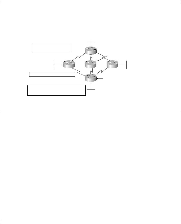
Figure 6-5 shows the typical sequence used by two EIGRP routers that connect to the same subnet. They discover each other as neighbors, and they reliably exchange full routing information. The process is different from OSPF, but the same goal of reliably ensuring that all neighbors receive all routing information is achieved. EIGRP sends and receives EIGRP hello packets to ensure that the neighbor is still up and working—like OSPF, but with a
Balanced Hybrid Routing Protocol and EIGRP Concepts 199
different Hello packet than OSPF. When link status changes, or new subnets are discovered, reliable routing updates are sent, but only with the new information—again, like OSPF.
Figure 6-5 Sequence of Events for EIGRP Exchange of Routing Information
|
|
|
|
|
|
|
|
|
|
|
|
|
|
|
B |
|
|
|
|
|
|
|
|
|
|||
|
|
|
|
|
|
|
A |
|
|
||||
|
|
|
|
|
|
|
|
|
|
|
|
|
|
|
|
|
|
|
|
|
|
|
|
|
|
||
|
Neighbor Discovery |
|
|
|
|
|
Neighbor Discovery |
|
|||||
|
|
|
|
|
|
Reliable |
|
|
|
|
|
|
|
|
|
|
|
|
|
|
|
|
|
|
|
||
|
|
|
|
|
|
|
|
|
|
|
|
||
|
Full Routing Update |
|
|
Full Routing Update |
|
||||||||
|
|
Update |
|
||||||||||
|
|
|
|
|
|
|
|
|
|
|
|||
|
|
|
|
|
|
|
|
|
|
||||
|
|
|
|
|
|
|
|
|
|
||||
|
Continuous Hellos |
|
|
|
|
|
Continuous Hellos |
|
|||||
|
|
|
|
|
|
|
|
|
|
||||
|
|
|
|
|
|
|
|
|
|
|
|||
|
|
|
|
|
|
|
|
|
|||||
Partial Updates (Status Changes |
|
|
|
|
Partial Updates (Status Changes |
||||||||
and New Subnet Info) |
|
|
|
|
and New Subnet Info) |
||||||||
|
|
|
|
|
|
|
|
|
|
|
|
|
|
EIGRP uses a formula based on bandwidth and delay to calculate the metric associated with a route. Sound familiar? It’s the same formula used by IGRP, but the number is multiplied by 256 to accommodate calculations when very high bandwidth values are used. Other than that, the actual metric calculation is the same as IGRP.
EIGRP Loop Avoidance
Loop avoidance poses one of the most difficult problems with any dynamic routing protocol. Distance vector protocols overcome this problem with a variety of tools, some of which create a large portion of the minutes-long convergence time after a link failure. Link-state protocols overcome this problem by having each router keep a full topology of the network, so that by running a rather involved mathematical model, a router can avoid any loops.
EIGRP avoids loops by keeping some basic topological information but not full information. When a router learns multiple routes to the same subnet, it puts the best route in the routing table. (EIGRP follows the same rules about adding multiple equal-metric routes as does IGRP. For this next discussion, I am assuming that if multiple routes to the same destination are found, one of the routes has the lowest metric, and only one route is added to the routing table.) Of the other suboptimal routes, some may be used immediately if the currently-best route fails, without fear of having a loop occur. EIGRP runs a simple algorithm to identify which routes could be used immediately after a route failure, without causing a loop. EIGRP then keeps these loop-free backup routes in its topology table and uses them if the currentlybest route fails.
200 Chapter 6: OSPF and EIGRP Concepts and Configuration
Figure 6-6 illustrates how EIGRP figures out which routes can be used after a route fails without causing loops.
Figure 6-6 Successors and Feasible Successors with EIGRP
Router E Calculates Metrics for Each Route:
Route Through Router B — 19,000
Route Through Router C — 17,500
Route Through Router D — 14,000


 Subnet 1 Metric 15,000
B
Subnet 1 Metric 13,000
Subnet 1
E C A
Router E Routing Table
Subnet 1 Metric 14,000, Through Router D
Subnet 1 Metric 10,000
D
Router E Topology Table for Subnet 1
Route Through Router D — Successor
Route Through Router C — Feasible Successor
(C’s Metric is 13,000, which Is Less than E’s Metric)
In the figure, Router E learns three routes to Subnet 1, from Routers B, C, and D. After calculating each route’s metric based on bandwidth and delay information received in the routing update, Router E finds that the route through Router D has the lowest metric, so Router E adds that route to its routing table, as shown.
EIGRP builds a topology table that includes the currently-best route plus the alternative routes that would not cause loops if they were used when the currently-best route through Router D failed. EIGRP calls the best route (the route with the lowest metric) the successor. Any backup routes that could be used without causing a loop are called feasible successors. In Figure 6-6, the route through Router C would not cause a loop, so Router E lists the route through Router C as a feasible successor. Router E thinks that using the route through Router B could cause a loop, so that route is not listed as a feasible successor.
EIGRP decides if a route can be a feasible successor if the computed metric for that route on the neighbor is less than its own computed metric. For example, Router E computes a metric of 14,000 on its best route (through Router D). Router C’s computed metric is lower than 14,000 (it’s 13,000), so Router E believes that if the existing route failed using the route to Subnet 1, through Router C, it would not cause a loop. As a result, Router E adds a route through Router C to the topology table as a feasible successor route. Conversely, Router B’s computed metric is 15,000, which is larger than Router E’s computed metric of 14,000, so Router E does not consider the route through Router B a feasible successor.
If the route to Subnet 1 through Router D fails, Router E can immediately put the route through Router C into the routing table, without fear of creating a loop. Convergence occurs almost instantly in this case.

OSPF Configuration 201
When a route fails and the route has no feasible successor, EIGRP uses a distributed algorithm called Diffusing Update Algorithm (DUAL). DUAL sends queries looking for a loop-free route to the subnet in question. When the new route is found, DUAL adds it to the routing table.
EIGRP Summary
EIGRP converges quickly while avoiding loops. EIGRP does not have the same scaling issues as link-state protocols, so no extra design effort is required. EIGRP takes less memory and processing than link-state protocols.
EIGRP converges much more quickly than do distance vector protocols, mainly
because EIGRP does not need the loop-avoidance features that slow down distance vector convergence. By sending only partial routing updates, after full routing information has been exchanged, EIGRP reduces overhead on the network.
The only significant disadvantage of EIGRP is that it is a Cisco-proprietary protocol. So, if you want to be prepared to use multiple vendors’ routers in a network, you should probably choose an alternative routing protocol. Alternatively, you could use EIGRP in the Cisco routers and OSPF in the others and perform a function called route redistribution, in which a router exchanges routes between the two routing protocols inside the router.
Table 6-3 summarizes some of the key comparison points between EIGRP, IGRP, and OSPF.
Table 6-3 EIGRP Features Compared to OSPF and IGRP
Feature |
EIGRP |
IGRP |
OSPF |
|
|
|
|
Discovers neighbors before exchanging routing information |
Yes |
No |
Yes |
|
|
|
|
Builds some form of topology table in addition to adding |
Yes |
No |
Yes |
routes to the routing table |
|
|
|
|
|
|
|
Converges quickly |
Yes |
No |
Yes |
|
|
|
|
Uses metrics based on bandwidth and delay by default |
Yes* |
Yes |
No |
Sends full routing information on every routing update cycle |
No |
Yes |
No |
|
|
|
|
Requires distance vector loop-avoidance features |
No |
Yes |
No |
|
|
|
|
Public standard |
No |
No |
Yes |
|
|
|
|
*EIGRP uses the same metric as IGRP, except that EIGRP scales the metric by multiplying by 256.
OSPF Configuration
OSPF includes many configuration options as a result of its complexity. Tables 6-4 and 6-5 summarize the OSPF configuration and troubleshooting commands, respectively.

202 Chapter 6: OSPF and EIGRP Concepts and Configuration
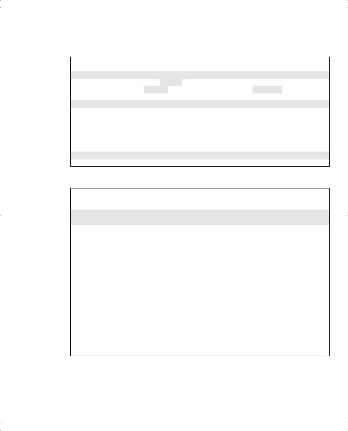
Table 6-4 IP OSPF Configuration Commands
|
Command |
Configuration Mode |
|
|
|
|
|
|
router ospf process-id |
Global |
|
|
|
|
|
|
network ip-address wildcard-mask area area-id |
Router subcommand |
|
|
|
|
|
|
ip ospf cost interface-cost |
Sets the OSPF cost associated with the |
|
|
|
interface |
|
|
|
|
|
|
bandwidth bandwidth |
Sets the interface bandwidth, from which |
|
|
|
OSPF derives the cost based on the |
|
|
|
formula 108 / bandwidth |
|
Table 6-5 |
IP OSPF EXEC Commands |
|
|
|
|
|
|
|
Command |
|
Description |
|
|
|
|
|
show ip route [ip-address [mask] [longer-prefixes]] | |
|
Shows the entire routing table, or a |
|
[protocol [process-id]] |
|
subset if parameters are entered. |
|
|
|
|
|
show ip protocols |
|
Shows routing protocol parameters |
|
|
|
and current timer values. |
|
|
|
|
|
show ip ospf interface |
|
Lists the area in which the interface |
|
|
|
resides, and neighbors adjacent on this |
|
|
|
interface. |
|
|
|
|
|
show ip ospf neighbor |
|
Lists neighbors and current status with |
|
|
|
neighbors, per interface. |
|
|
|
|
|
show ip route ospf |
|
Lists routes in the routing table learned |
|
|
|
by OSPF. |
|
|
|
|
|
debug ip ospf events |
|
Issues log messages for each OSPF |
|
|
|
packet. |
|
|
|
|
|
debug ip ospf packet |
|
Issues log messages describing the |
|
|
|
contents of all OSPF packets. |
|
|
|
|
This section includes two sample configurations using the same network diagram. The first example shows a configuration with a single OSPF area, and the second example shows multiple areas, along with some show commands.
OSPF Single-Area Configuration
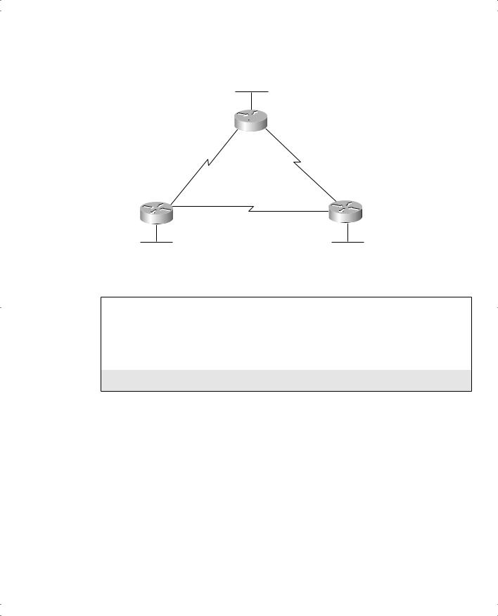
When only a single area is used, OSPF configuration differs only slightly from RIP and IGRP configuration. The best way to describe the configuration, and the differences with
the configuration of the other routing protocols, is to use an example. Figure 6-7 shows a sample network, and Example 6-1 shows the configuration on Albuquerque.
OSPF Configuration 203
Figure 6-7 Sample Network for OSPF Single-Area Configuration
Subnet 10.1.1.0
E0/0

 Albuquerque
S0/0 S0/1
|
.0 |
|
.4 |
|
.1 |
Subnet |
10 |
|
Subnet
10 . 1 . 6 . 0
S0/0 S0/1 |
S0/0 |
Subnet 10.1.5.0 |
|
|
S0/1 |
|
Seville |
E0/0 Subnet 10.1.2.0 |
E0/0 Subnet 10.1.3.0 |
Example 6-1 OSPF Single-Area Configuration on Albuquerque
interface ethernet 0/0
ip address 10.1.1.1 255.255.255.0 interface serial 0/0
ip address 10.1.4.1 255.255.255.0 interface serial 0/1
ip address 10.1.6.1 255.255.255.0
!
router ospf 1
network 10.0.0.0 0.255.255.255 area 0
The configuration correctly enables OSPF on all three interfaces on Albuquerque. First, the router ospf 1 global command puts the user in OSPF configuration mode. The router ospf command has a parameter called the OSPF process-id. In some instances, you might want to run multiple OSPF processes in a single router, so the router command uses the process-id to distinguish between the processes. Although the process-id used on the three routers is the same, the actual value is unimportant, and the numbers do not have to match on each router.
The network command tells Albuquerque to enable OSPF on all interfaces that match the network command and, on those interfaces, to place the interfaces into Area 0. The
OSPF network command matches interfaces differently than does the network command for RIP and IGRP. The OSPF network command includes a parameter called the wildcard mask. The wildcard mask works just like the wildcard mask used with Cisco access control lists (ACLs), which are covered in more depth in Chapter 12, “IP Access Control List Security.”

204 Chapter 6: OSPF and EIGRP Concepts and Configuration
The wildcard mask represents a 32-bit number. When the mask has a binary 1 in one of the bit positions, that bit is considered a wildcard bit, meaning that the router should not care what binary value is in the corresponding numbers. For that reason, binary 1s in the wildcard mask are called don’t care bits. If the wildcard mask bit is 0 in a bit position, the corresponding bits in the numbers being compared must match. You can think of these bits as the do care bits. So, the router must examine the two numbers and make sure that the values match for the bits that matter—in other words, the do care bits.
For instance, the wildcard mask in Example 6-1 is 0.255.255.255. When converted to binary, this number is 0000 0000 1111 1111 1111 1111 1111 1111—in other words, eight 0s and 24 1s. The network command tells Cisco IOS software to compare 10.0.0.0, which is the number in the network command, to the IP addresses of each interface on the router. The wildcard mask tells Cisco IOS software to compare only the first octet; the last three octets are wildcards, and anything matches. So, all three interface IP addresses are matched.
Example 6-2 shows an alternative configuration for Albuquerque that also enables OSPF on every interface. In this case, the IP address for each interface is matched with a different network command. The wildcard mask of 0.0.0.0 means that all 32 bits must be compared, and they must match—so the network commands include the specific IP address of each interface, respectively. Many people prefer this style of configuration in production networks, because it removes any ambiguity as to the interfaces on which OSPF is running.
Example 6-2 OSPF Single-Area Configuration on Albuquerque Using Three network Commands
interface ethernet 0/0
ip address 10.1.1.1 255.255.255.0 interface serial 0/0
ip address 10.1.4.1 255.255.255.0 interface serial 0/1
ip address 10.1.6.1 255.255.255.0
!
router ospf 1
network 10.1.1.1 0.0.0.0 area 0 network 10.1.4.1 0.0.0.0 area 0 network 10.1.6.1 0.0.0.0 area 0
OSPF Configuration with Multiple Areas
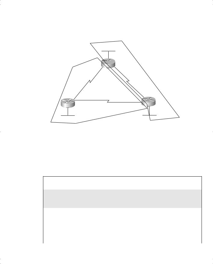
Configuring OSPF with multiple areas is simple once you understand OSPF configuration in a single area. Designing the OSPF network by making good choices as to which subnets should be placed in which areas is the hard part! After the area design is complete, the configuration is easy. For instance, consider Figure 6-8, which shows some subnets in Area 0 and some in Area 1.
OSPF Configuration 205
Figure 6-8 Multiarea OSPF Network
Area 0
Subnet 10.1.1.0
Area 0

 Albuquerque
S0/0 S0/1
|
.0 |
|
.4 |
|
.1 |
Subnet |
10 |
|
Subnet
10 . 1 . 6 . 0
S0/0 S0/1 |
S0/0 |
Subnet 10.1.5.0 |
|
Yosemite |
S0/1 |
Seville |
|
Subnet 10.1.2.0 |
Subnet 10.1.3.0 |
Multiple areas are not needed in such a small network, but two areas are used in this example to show the configuration. Note that Albuquerque and Seville are both ABRs, but Yosemite is totally inside area 1, so it is not an ABR.
Examples 6-3 and 6-4 show the configuration on Albuquerque and Yosemite, along with several show commands.
Example 6-3 OSPF Multiarea Configuration and show Commands on Albuquerque
!
! Only the OSPF configuration is shown to conserve space
!
router ospf 1
network 10.1.1.1 0.0.0.0 area 0 network 10.1.4.1 0.0.0.0 area 1 network 10.1.6.1 0.0.0.0 area 0
Albuquerque#show ip route
Codes: C - connected, S - static, I - IGRP, R - RIP, M - mobile, B - BGP
D - EIGRP, EX - EIGRP external, O - OSPF, IA - OSPF inter area
N1 - OSPF NSSA external type 1, N2 - OSPF NSSA external type 2
E1 - OSPF external type 1, E2 - OSPF external type 2, E - EGP
i - IS-IS, L1 - IS-IS level-1, L2 - IS-IS level-2, ia - IS-IS inter area * - candidate default, U - per-user static route, o - ODR
P - periodic downloaded static route
continues

206 Chapter 6: OSPF and EIGRP Concepts and Configuration
Example 6-3 OSPF Multiarea Configuration and show Commands on Albuquerque (Continued)
Gateway of last resort is not set
10.0.0.0/24 is subnetted, 6 subnets
O10.1.3.0 [110/65] via 10.1.6.3, 00:01:04, Serial0/1
O10.1.2.0 [110/65] via 10.1.4.2, 00:00:39, Serial0/0 C 10.1.1.0 is directly connected, Ethernet0/0
C 10.1.6.0 is directly connected, Serial0/1
O10.1.5.0 [110/128] via 10.1.4.2, 00:00:39, Serial0/0 C 10.1.4.0 is directly connected, Serial0/0
Albuquerque#show ip route ospf
10.0.0.0/24 is subnetted, 6 subnets
O10.1.3.0 [110/65] via 10.1.6.3, 00:01:08, Serial0/1
O10.1.2.0 [110/65] via 10.1.4.2, 00:00:43, Serial0/0
O10.1.5.0 [110/128] via 10.1.4.2, 00:00:43, Serial0/0 Albuquerque#show ip ospf neighbor
Neighbor ID |
Pri |
State |
|
Dead Time |
Address |
Interface |
|
10.1.6.3 |
|
1 |
FULL/ |
- |
00:00:35 |
10.1.6.3 |
Serial0/1 |
10.1.5.2 |
|
1 |
FULL/ |
- |
00:00:37 |
10.1.4.2 |
Serial0/0 |
|
|
|
|
|
|
|
|
Albuquerque#show ip ospf interface
Serial0/1 is up, line protocol is up
Internet Address 10.1.6.1/24, Area 0
Process ID 1, Router ID 10.1.6.1, Network Type POINT_TO_POINT, Cost: 64 Transmit Delay is 1 sec, State POINT_TO_POINT,
Timer intervals configured, Hello 10, Dead 40, Wait 40, Retransmit 5 Hello due in 00:00:07
Index 2/3, flood queue length 0
Next 0x0(0)/0x0(0)
Last flood scan length is 2, maximum is 2
Last flood scan time is 0 msec, maximum is 0 msec
Neighbor Count is 1, Adjacent neighbor count is 1
Adjacent with neighbor 10.1.6.3
Suppress hello for 0 neighbor(s)
Ethernet0/0 is up, line protocol is up
Internet Address 10.1.1.1/24, Area 0
Process ID 1, Router ID 10.1.6.1, Network Type BROADCAST, Cost: 10
Transmit Delay is 1 sec, State DR, Priority 1
Designated Router (ID) 10.1.6.1, Interface address 10.1.1.1
No backup designated router on this network
Timer intervals configured, Hello 10, Dead 40, Wait 40, Retransmit 5 Hello due in 00:00:08
Index 1/1, flood queue length 0
Next 0x0(0)/0x0(0)
Last flood scan length is 0, maximum is 0
Last flood scan time is 0 msec, maximum is 0 msec
OSPF Configuration 207
Example 6-3 OSPF Multiarea Configuration and show Commands on Albuquerque (Continued)
Neighbor Count is 0, Adjacent neighbor count is 0
Suppress hello for 0 neighbor(s)
Serial0/0 is up, line protocol is up
Internet Address 10.1.4.1/24, Area 1
Process ID 1, Router ID 10.1.6.1, Network Type POINT_TO_POINT, Cost: 64
Transmit Delay is 1 sec, State POINT_TO_POINT,
Timer intervals configured, Hello 10, Dead 40, Wait 40, Retransmit 5
Hello due in 00:00:01
Index 1/2, flood queue length 0
Next 0x0(0)/0x0(0)
Last flood scan length is 1, maximum is 1
Last flood scan time is 0 msec, maximum is 0 msec
Neighbor Count is 1, Adjacent neighbor count is 1
Adjacent with neighbor 10.1.5.2
Suppress hello for 0 neighbor(s)
Example 6-4 OSPF Multiarea Configuration and show Commands on Yosemite
!
! Only the OSPF configuration is shown to conserve space
!
router ospf 1
network 10.0.0.0 area 1
Yosemite#show ip route
Codes: C - connected, S - static, I - IGRP, R - RIP, M - mobile, B - BGP
D - EIGRP, EX - EIGRP external, O - OSPF, IA - OSPF inter area
N1 - OSPF NSSA external type 1, N2 - OSPF NSSA external type 2
E1 - OSPF external type 1, E2 - OSPF external type 2, E - EGP
i - IS-IS, L1 - IS-IS level-1, L2 - IS-IS level-2, ia - IS-IS inter area * - candidate default, U - per-user static route, o - ODR
P - periodic downloaded static route
Gateway |
of last resort is not set |
|||
10.0.0.0/24 |
is subnetted, 6 subnets |
|||
IA |
10.1.3.0 |
[110/65] |
via |
10.1.5.1, 00:00:54, Serial0/1 |
IA |
10.1.1.0 |
[110/65] |
via |
10.1.4.1, 00:00:49, Serial0/0 |
C10.1.2.0 is directly connected, Ethernet0/0
C10.1.5.0 is directly connected, Serial0/1
IA |
10.1.6.0 [110/128] via 10.1.4.1, 00:00:38, Serial0/0 |
C10.1.4.0 is directly connected, Serial0/0
The configuration only needs to show the correct area number on the network command matching the appropriate interfaces. For instance, the network 10.1.4.1 0.0.0.0 area 1 command matches Albuquerque’s Serial 0/0 interface IP address, placing that interface in
Area 1. The network 10.1.6.1 0.0.0.0 area 0 and network 10.1.1.1 0.0.0.0 area 0 commands

208 Chapter 6: OSPF and EIGRP Concepts and Configuration
place Serial 0/1 and Ethernet 0/0, respectively, in Area 0. Unlike Example 6-1, Albuquerque cannot be configured to match all three interfaces with a single network command, because one interface (Serial 0/0) is in a different area than the other two interfaces.
The show ip route ospf command just lists OSPF-learned routes, as opposed to the entire IP routing table. The show ip route command lists all three connected routes, as well as the three OSPF learned routes. Note that Albuquerque’s route to 10.1.2.0 has the O designation beside it, meaning intra-area, because that subnet resides in Area 1, and Albuquerque is part of Area 1 and Area 0.
In Example 6-4, notice that the OSPF configuration in Yosemite requires only a single network command. Because all interfaces in Yosemite are in Area 1, and all three interfaces are in network 10.0.0.0, the command can just match all IP addresses in network 10.0.0.0 and put them in Area 1. Also note that the routes learned by Yosemite from the other two routers show up as interarea (IA) routes, because those subnets are in Area 0, and Yosemite is in Area 1.
The OSPF topology database includes information about routers and the subnets, or links, to which they are attached. To identify the routers in the neighbor table’s topology database, OSPF uses a router ID (RID) for each router. A router’s OSPF RID is that router’s highest IP address on a physical interface when OSPF starts running. Alternatively, if a loopback interface has been configured, OSPF uses the highest IP address on a loopback interface for the RID, even if that IP address is lower than some physical interface’s IP address. Also, you can set the OSPF RID using the router-id command in router configuration mode.
NOTE If you’re not familiar with it, a loopback interface is a special virtual interface in a Cisco router. If you create a loopback interface using the interface loopback x command, where x is a number, that loopback interface is up and operational as long as the router IOS is up and working. You can assign an IP address to a loopback interface, you can ping the address, and you can use it for several purposes—including having a loopback interface IP address as the OSPF router ID.
Many commands refer to the OSPF RID, including the show ip ospf neighbor command. This command lists all the neighbors, using the neighbors’ RIDs to identify them. For instance, in Example 6-3, the first neighbor in the output of the show ip ospf neighbor command lists Router ID 10.1.5.2, which is Yosemite’s RID.
Finally, the show ip ospf interface command lists more-detailed information about OSPF operation on each interface. For instance, this command lists the area number, OSPF cost, and any neighbors known on each interface. The timers used on the interface, including the Hello and dead timer, are also listed.
EIGRP Configuration 209
OSPF uses the cost to determine the metric for each route. You can set the cost value on an interface using the ip ospf cost x interface subcommand. You can also set the OSPF cost of an interface using the bandwidth interface subcommand. If you do not set an interface’s cost, IOS defaults to use the formula 108 / bandwidth, where bandwidth is the interface’s bandwidth. For instance, Cisco IOS software defaults to a bandwidth of 10,000 (the unit in the bandwidth command is kbps, so 10,000 means 10 Mbps) on Ethernet interfaces, so the default cost is 108 / 107, or 10. Higher-speed serial interfaces default to a bandwidth of 1544, giving a default cost of 108 / 1,544,000, which is rounded to 64, as shown in the example. If you change the interface’s bandwidth, you change the OSPF cost as well.
You might have noticed that the cost for a Fast Ethernet interface (100 Mbps) is calculated as a cost of 1. For Gigabit interfaces (1000 Mbps), the calculation yields .1, but only integer values can be used, so OSPF uses a cost of 1 for Gigabit interfaces as well. So Cisco lets you change the reference bandwidth, which is the value in the numerator of the calculation in the preceding paragraph. For instance, using the router OSPF subcommand auto-cost referencebandwidth 1000, you change the numerator to 1000 Mbps, or 109. The calculated cost on a Gigabit interface is then 1, and the cost on a Fast Ethernet is 10.
EIGRP Configuration
If you remember how to configure IGRP, EIGRP configuration is painless. You configure EIGRP exactly like IGRP, except that you use the eigrp keyword instead of the igrp keyword in the router command.
Tables 6-6 and 6-7 summarize the EIGRP configuration and troubleshooting commands, respectively. After these tables, you will see a short demonstration of EIGRP configuration, along with show command output.
Table 6-6 IP EIGRP Configuration Commands
Command |
Configuration Mode |
|
|
router eigrp autonomous-system |
Global |
|
|
network network-number |
Router subcommand |
|
|
maximum-paths number-paths |
Router subcommand |
|
|
variance multiplier |
Router subcommand |
|
|
traffic-share {balanced | min} |
Router subcommand |
|
|


EIGRP Configuration 211
Example 6-5 Sample Router Configuration with RIP Partially Enabled (Continued)
10.0.0.0/24 is subnetted, 6 subnets
D10.1.3.0 [90/2172416] via 10.1.6.3, 00:00:47, Serial0/1
D10.1.2.0 [90/2172416] via 10.1.4.2, 00:00:47, Serial0/0
D10.1.5.0 [90/2681856] via 10.1.6.3, 00:00:49, Serial0/1 [90/2681856] via 10.1.4.2, 00:00:49, Serial0/0
Albuquerque#show ip eigrp neighbors |
|
|
|
|
|
||||||
IP-EIGRP neighbors for process 1 |
|
|
|
|
|
|
|
||||
H |
Address |
|
|
Interface |
Hold Uptime |
SRTT |
RTO |
Q |
Seq Type |
||
|
|
|
|
|
|
|
(sec) |
(ms) |
|
Cnt Num |
|
|
|
|
|
|
|
|
|
|
|
|
|
0 |
10.1.4.2 |
|
|
Se0/0 |
|
|
11 00:00:54 |
32 |
200 |
0 |
4 |
1 |
10.1.6.3 |
|
|
Se0/1 |
|
|
12 00:10:36 |
20 |
200 |
0 |
24 |
Albuquerque#show ip eigrp interfaces |
|
|
|
|
|
||||||
IP-EIGRP interfaces for process 1 |
|
|
|
|
|
|
|
||||
|
|
|
|
Xmit Queue |
Mean |
Pacing Time |
Multicast |
|
Pending |
||
Interface |
Peers |
Un/Reliable |
SRTT |
Un/Reliable |
Flow Timer |
|
Routes |
||||
|
|
|
|
|
|
|
|
|
|
||
Et0/0 |
0 |
|
0/0 |
0 |
0/10 |
|
0 |
|
0 |
||
Se0/0 |
1 |
|
0/0 |
32 |
0/15 |
|
50 |
|
0 |
||
Se0/1 |
1 |
|
0/0 |
20 |
0/15 |
|
95 |
|
0 |
||
|
|
|
|
|
|
|
|
|
|
|
|
For EIGRP configuration, all three routers must use the same AS number on the router eigrp command. For instance, they all use router eigrp 1 in this example. The actual number used doesn’t really matter, as long as it is the same number on all 3 routers. The network 10.0.0.0 command enables EIGRP on all interfaces whose IP addresses are in network 10.0.0.0, which includes all three interfaces on Albuquerque. With the identical two EIGRP configuration statements on the other two routers, EIGRP is enabled on all three interfaces on those routers as well, because those interfaces are also in network 10.0.0.0.
The show ip route and show ip route eigrp commands both list the EIGRP-learned routes with a D beside them. D signifies EIGRP. The letter E was already being used for Exterior Gateway Protocol (EGP) when Cisco created EIGRP, so it chose the next-closest letter to denote EIGRP-learned routes. You can see information about EIGRP neighbors with the show ip eigrp neighbors command, and the number of active neighbors (called peers in the command output) with the show ip eigrp interfaces command, as seen in the last part of the example.