Only the second branch of the above solution is consistent with (9.2.113) from which the constraints (9.2.115) were derived. Restricting our attention to such a branch, the two magnetic charges pΣ are identified by (9.2.113) as it follows:

(9.2.117)

Equation (9.2.117) can now be inverted expressing the parameters y and σ in terms of the charges pΛ and of the value of the scalar field at infinity κ, ξ . The explicit inversion of the above formulae is quite involved and not relevant for our discussion, so we omit it.

If we calculate the limiting value taken by complex scalar field when τ → −∞

With a little bit of algebraic work one can verify that this value is actually the same as:

This is just the attractor mechanism. Independently from their values at infinity the scalar fields go to a fixed value at the horizon which depends only on the charges. The novelty, however, is that this horizon has a vanishing area. Indeed from the explicit form of the U (τ ) function we obtain:

This is consistent with the fact that the quartic invariant with such charges as those

9.2.11 Behavior of the Riemann Tensor in Regular Solutions

In order to better appreciate the approach to horizon in regular solutions it is convenient to study more in depth the solution based on the metric (9.2.87) and the scalar field (9.2.88), (9.2.89). As long as we do not mention the accompanying vector functions ZΛ(τ ) we do not know whether (9.2.87), (9.2.88), (9.2.89) describe the non-BPS or the BPS solution. Yet in both cases p, q are restricted to have the same sign which means equal sign for p2, q1 in the non-BPS case and opposite sign for the same charges in the BPS one. If we insert the explicit form of the warp factor

.

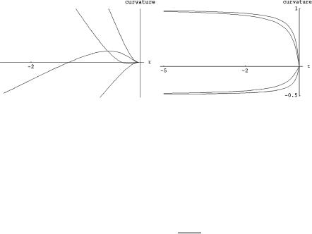
Fig. 9.2 Evolution of the four independent component of the curvature for the non-BPS and BPS solutions with ξ = 0, κ = 1, q = 2, p = 18 . In the picture on the left we see the behavior of the curvature near τ = 0 namely at asymptotic infinity where they go all to zero. In the picture on the right we see the asymptotic behavior for large negative τ , namely near the horizon where the curvatures go to their constant values and the space degenerates into the direct product AdS2 × S2

(9.2.87) in the expression (9.2.34) for the independent component of the Riemann tensor we can verify the following asymptotic behavior:

This has a profound meaning. The vanishing of all curvature components at radial infinity corresponds to the condition of asymptotic flatness which is a necessary boundary condition for physically meaningful black-holes. On the other hand the characteristic integer values of the Riemann tensor components obtained at the horizon correspond to the factorization of the four-dimensional geometry into the direct product AdS2 × S2. The interpretation of the regular black-holes as an interpolating soliton between two different vacua of supergravity is thus manifest. At τ = 0 we have the vacuum Mink4. At the horizon we have the vacuum AdS2 × S2 which requires an appropriate form of the electromagnetic fields. In Fig. 9.2 we present the behavior of the four functions in a numerical case-study where the approach to the asymptotic constant values at the horizon can be clearly seen.

9.3Flux Vacua of M-Theory and Manifolds of Restricted Holonomy

The next instance of supergravity solutions that we consider has been announced in the introduction. We will focus on compactified vacua solutions of M-theory. By vacuum it is meant that four of the eleven dimensions of M-theory correspond to those of a maximally symmetric manifold, (Minkowski, de Sitter or anti de Sitter space). Compactification instead occurs if the remaining seven dimensions are rolled up into a compact 7-manifold whose size is fixed by its average curvature radius.

374 9 Supergravity: An Anthology of Solutions

the curvature superfield. This latter is determined from the expansion of the inner components of the 4-form field strength Fa1...a4 . From the (6.4.6) we obtain:

This shows that the gravitino field strength appears at first order in the θ -expansion of the curvature superfield. Next we consider the spinor derivative of the gravitino field strength itself. Using the normalization which streams from the following definition:

The tensor-matrix Kab is of key importance in the discussion of compactifications. If it vanishes on a given background it means that the gravitino field strength can be consistently put to zero to all orders in θ s and on its turn this implies that the 4- field strength can be chosen constant to all orders in θ s. This is the case of maximal unbroken supersymmetry. In this case all curvature components of the Free Differential Algebra can be chosen constant and we have a superspace whose geometry is purely described by Maurer Cartan forms of some super coset.

On the other hand if Kab , that we name the holonomy tensor does not vanish this implies that both ρab and Fabcd have some non-trivial θ -dependence and cannot be chosen constant. In this case the geometry of superspace is not described by simple Maurer Cartan forms of some supercoset, since the curvatures of the FDA are not pure constants. This is the case of fully or partially broken SUSY and it is the case we explore. In the AdS4 × (G /H )7 compactifications it turns out that the matrix Kab is related to the holonomy tensor of the internal manifold (G /H )7.

Let us finally work out the spinor derivative of the Riemann tensor. Defining:

The matrix Kab and the spinor Λabmn are the crucial objects we are supposed to compute in each compactification background.

9.3.2Flux Compactifications of M-Theory on AdS4 × M7

Backgrounds

We are interested in compactified backgrounds where the 11-dimensional bosonic manifold is of the form:

M4 denoting a four-dimensional maximally symmetric manifold whose coordinates we denote xμ and M7 a 7-dimensional compact manifold whose parameters we denote yI . Furthermore we assume that in any configuration of the compactified theory the eleven dimensional vielbein is split as follows:

where Er (x) is a purely x-dependent 4-dimensional vielbein, W α (x) is an x- dependent 1-form on x-space describing the Kaluza Klein vectors and the purely x-dependent 7 × 7 matrix Φαβ (x) encodes part of the scalar fields of the compactified theory, namely the internal metric moduli. From these assumptions it follows that the bosonic field strength is expanded as follows:

F[(Bosonic)4] ≡ F [4](x) + Fα[3](x) V α + Fαβ[2](x) V α V β

+ Fαβγ[1] (x) V α V β V γ + Fαβγ[0] δ (x) V α V β V γ V δ

(9.3.16)

[p]

where Fα1...α4−p (x) are x-space p-forms depending only on x.

In bosonic backgrounds with a space-time geometry of the form (9.3.14), the family of configurations (9.3.15) must satisfy the condition that by choosing:

we obtain an exact bona fide solution of the eleven-dimensional field equations of M-theory.

There are three possible 4-dimensional maximally symmetric Lorentzian manifolds

In any case Lorentz invariance imposes (9.3.18), (9.3.19), (9.3.20) while translation invariance imposes that the vacuum expectation value of the scalar fields Φαβ (x) should be a constant matrix

We are interested in 7-manifolds that preserve some residual supersymmetry in D = 4. This relates to the holonomy of M7 which has to be restricted in order to allow for the existence of Killing spinors. In the next subsection we summarize the basic results from the literature on this topic.

9.3.3M-Theory Field Equations and 7-Manifolds of Weak G2 Holonomy i.e. Englert 7-Manifolds

In order to admit at least one Killing spinor or more, the 7-manifold M7 necessarily must have a (weak) holonomy smaller than SO(7): at most G2. The qualification weak refers to the definition of holonomy appropriate to compactifications on AdS4 × M7 while the standard definition of holonomy is appropriate to compactifications on Ricci flat backgrounds Mink4 × M7. To explain in contemporary language these concepts that were discovered in the eighties we have to recall the notion of G-structures. Indeed in the recent literature about flux compactifications the key geometrical notion exploited by most authors is precisely that of G-structures [22].

Following, for instance, the presentation of [22], if Mn is a differentiable man-

π π

ifold of dimension n, T Mn → Mn its tangent bundle and F Mn → Mn its frame bundle, we say that Mn admits a G-structure when the structural group of F Mn is reduced from the generic GL(n, R) to a proper subgroup G GL(n, R). Generically, tensors on Mn transform in representations of the structural group GL(n, R). If a G-structure reduces this latter to G GL(n, R), then the decomposition of an irreducible representation of GL(n, R), pertaining to a certain tensor tp , with respect to the subgroup G may contain singlets. This means that on such a manifold Mn there may exist a certain tensor tp which is G-invariant, and therefore globally defined. As recalled in [22] existence of a Riemannian metric g on Mn is equivalent to a reduction of the structural group GL(n, R) to O(n), namely to an O(n)-structure. Indeed, one can reduce the frame bundle by introducing orthonormal frames, the vielbein eI , and, written in these frames, the metric is the O(n) invariant tensor

δI J . Similarly orientability corresponds to an SO(n)-structure and the existence of spinors on spin manifolds corresponds to a Spin(n)-structure.

In the case of seven dimensions, an orientable Riemannian manifold M7, whose frame bundle has generically an SO(7) structural group, admits a G2-structure if and only if, in the basis provided by the orthonormal frames Bα , there exists an antisymmetric 3-tensor φαβγ δ satisfying the algebra of the octonionic structure constants:

which is invariant, namely it is the same in all local trivializations of the SO(7) frame bundle. This corresponds to the algebraic definition of G2 as that subgroup of SO(7) which acts as an automorphism group of the octonion algebra. Alternatively G2 can be defined as the stability subgroup of the 8-dimensional spinor representation of SO(7). Hence we can equivalently state that a manifold M7 has a G2-structure if there exists at least an invariant spinor η, which is the same in all local trivializations of the Spin(7) spinor bundle.

In terms of this invariant spinor the invariant 3-tensor φρσ κ

and (9.3.26) provides the relation between the two definitions of the G2-structure. On the other hand the manifold has not only a G2-structure, but also G2-

holonomy if the invariant three-tensor φαβκ is covariantly constant, namely:

where the 1-form Bαβ is the spin connection of M7. Alternatively the manifold has G2-holonomy if the invariant spinor η is covariantly constant, namely if:

where τ α (α = 1, . . . , 7) are the 8 × 8 gamma matrices of the SO(7) Clifford algebra (see footnote). The relation between the two definitions (9.3.27) and (9.3.28) of G2- holonomy is the same as for the two definitions of the G2-structure, namely it is given by (9.3.26). As a consequence of its own definition a Riemannian 7-manifold with G2 holonomy is Ricci flat. Indeed the integrability condition of (9.3.28) yields:

6By τ α we denote the gamma matrices in 7-dimensions, satisfying the Clifford algebra {τ α , τ β } = −δαβ . With the symbol τ α1...αn we denote, as usual, the antisymmetrized product of n such matrices.

αβ

where R γ δ is the Riemann tensor of M7. From (9.3.29), by means of a few simple algebraic manipulations one obtains two results:

• The curvature 2-form

which projects out the 7 of G2 from the 21 of SO(7) and leaves with the adjoint 14.

• The internal Ricci tensor is zero:

Next we consider the bosonic field equations of M-theory, namely the first and the last of (6.4.9). We make the compactification ansatz (9.3.14) where M4 is one of the three possibilities mentioned in (9.3.23) and all of (9.3.18)–(9.3.22) hold true. Then we split the rigid index range as follows:

and by following the conventions employed in [23] and using the results obtained in the same paper, we conclude that the compactification ansatz reduces the system of the first and last of (6.4.9) to the following one:

Equation (9.3.35) states that the internal manifold M7 must be an Einstein space. Equations (9.3.36) and (9.3.37) state that there is a flux of the four-form both on 4-dimensional space-time M4 and on the internal manifold M7. The parameter e, which fixes the size of the flux on the four-dimensional space and was already introduced in (9.3.21), is called the Freund-Rubin parameter [24]. As we are going to show, in the case that a non-vanishing F is required to exist, (9.3.38) and (9.3.39), are equivalent to the assertion that the manifold M7 has weak G2 holonomy rather than G2-holonomy, to state it in modern parlance [25]. In paper [26],

manifolds admitting such a structure were instead named Englert spaces and the underlying notion of weak G2 holonomy was already introduced there with the different name of de Sitter SO(7)+ holonomy.

Indeed (9.3.39) which, in the language of the early eighties was named Englert equation [27] and which is nothing else but the first equation of (6.4.9), upon substitution of the Freund Rubin ansatz (9.3.36) for the external flux, can be recast in the following more revealing form: Let

be a the constant 4-form on M7 defined by our non-vanishing flux, and let

be its dual. Englert equation (9.3.39) is just the same as writing:

dΦ = 12eΦ

(9.3.42)

dΦ = 0

When the Freund Rubin parameter vanishes e = 0 we recognize in (9.3.42) the statement that our internal manifold M7 has G2-holonomy and hence it is Ricci flat. Indeed Φ is the G2 invariant and covariantly constant form defining G2-structure and G2-holonomy. On the other hand the case e = 0 corresponds to the weak G2 holonomy. Just as we reduced the existence of a closed three-form Φ to the existence of a G2 covariantly constant spinor satisfying (9.3.28) which allows to set the identification (9.3.26), in the same way (9.3.42) can be solved if and only if on M7 there exist a weak Killing spinor η satisfying the following defining condition:

where m is a numerical constant and e is the Freund-Rubin parameter, namely the only scale which at the end of the day will occur in the solution.

The integrability of the above equation implies that the Ricci tensor be proportional to the identity, namely that the manifold is an Einstein manifold and furthermore fixes the proportionality constant:

In case such a spinor exists, by setting:

These correspond to anti de Sitter space in 4-dimensions, whose radius is fixed by the Freund Rubin parameter e = 0 times any Einstein manifold in 7- dimensions with no internal flux, namely gαβγ δ = 0. In this case from (9.3.50) we uniquely obtain:

Einst. manif. weak G2 hol

These correspond to anti de Sitter space in 4-dimensions (e = 0) times a 7- dimensional Einstein manifold which is necessarily of weak G2 holonomy in order to support a consistent non-vanishing internal flux gαβγ δ . In this case combining (9.3.50) with the previous ones we uniquely obtain:

As we already mentioned in the introduction there exist several compact manifolds of weak G2 holonomy. In particular all the coset manifolds G /H of weak G2 holonomy were classified and studied in the Kaluza Klein supergravity age [23, 26, 28–35] and they were extensively reconsidered in the context of the AdS/CFT correspondence [36–40].

In the present section we present the supergauge completion, namely the extension to a convenient superspace containing all or a subset of the 32 fermionic coordinates θ s of the compactifications of the Freund Rubin type, namely on elevenmanifolds of the form:

with no internal flux gαβγ δ switched on. As it was extensively explained in [41] and further developed in [36–40], if the compact coset G /H admits N ≤ 8 Killing spinors ηA, namely N ≤ 8 independent solutions of (9.3.43) with m = 1, then the isometry group G is necessarily of the form:

where Gflavor is some appropriate Lie group. In this case the isometry supergroup of the considered M-theory background is: