space-time is homogeneous. In addition we need the same scale factor a(t) in all directions and this is the outcome of isotropy.

5.5.2Solution of the Cosmological Differential Equations for Dust and Radiation Without a Cosmological Constant

If we substitute the first integral given by the conservation law (5.5.3) into the first of the differential equations (5.4.12) we get:

The differential equation for the scale factor in the case of a radiation filled universe is immediately integrated and yields the following simple result:

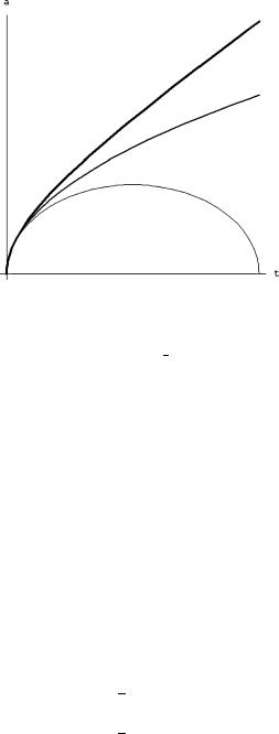
where the integration constant has been fixed by means of the boundary condition a(0) = 0 (see Fig. 5.17).

As it is evident from the above analytic form the solution for a positively curved

√

universe (κ = 1) makes sense only in the interval, 0 ≤ t ≤ 2 Cr where the function under square root is positive. Hence while for the open and flat universe (κ ≤ 0), the scale factor grows indefinitely and the expansion never ceases, the closed universe undergoes an expansion phase followed by a contraction one which finally concentrates again all the radiation into a single point with a diverging energy density.

Although the analytic form of the solution is slightly different, the qualitative behavior of the scale factor follows exactly the same pattern also in the case of a dust filled universe, as we demonstrate in the following subsections, separately analyzing the three cases.

Fig. 5.17 Evolution of the cosmological scale factor a(t) in the case of a radiation filled universe, for the three cases of positive (κ = 1), negative (κ = −1) and vanishing spatial curvature (κ = 0). The thickest line corresponds to the hyperbolic case (κ = −1) where, for late times, the scale factor grows asymptotically as a t . The medium thick line corresponds to the flat case where the late time asymptotic behavior of the scale factor is a √t . Finally the thinnest line correspond to the elliptic case (κ = 1), where the scale factor reaches a maximum and then contracts again to zero

5.5.2.1Parametric Solution in the Dust Case of a Positively Curved Universe κ = 1

We solve the differential equation pertaining to this case by means of a suitable change of variables. We introduce the new variable η and we set:

and hence, by straightforward integration, we find the parametric solution for the curve describing the evolution of the scale factor in the plane t, a:

a(η) = 1 Cd (1 − cos η)

2

(5.5.24)

t (η) = 1 Cd (η − sin η)

2

In Fig. 5.18 we show two instances of these evolutions. As one sees, in a positively curved universe, an initial expansion is always followed by a contraction phase.

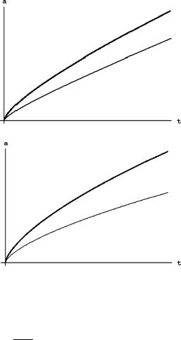
Fig. 5.19 Evolution of the cosmological scale factor a(t) in the case of an open

(κ = −1) dust universe. Also here the amplitude of the expansion depends on the total matter content of the universe codified by the constant Cd . The thicker line corresponds to the case

Cd = 1 while the thinner line corresponds to the case

Cd = 0.2

Fig. 5.20 Evolution of the cosmological scale factor a(t) in the case of a flat (κ = 0) dust universe. Also here the amplitude of the expansion depends on the total matter content of the universe codified by the constant Cd . The thicker line corresponds to the case Cd = 1 while the thinner line corresponds to the case Cd = 0.5

5.5.2.3 Parametric Solution in the Dust Case of a Spatially Flat Universe κ = 0

In the case of zero spatial curvature, (5.5.20) reduce, for a dust universe, to:

We conclude that also the flat, dust filled, universe expands indefinitely and the scale

In Fig. 5.21 we have compared the three kinds of behavior of the cosmological scale factor for the positively, negatively curved and flat, dust filled universe.

As one sees the qualitative behavior is exactly the same as in the case of radiation. Such behavior changes dramatically when we consider the case of universes with a positive space-time curvature, in particular the maximally symmetric de Sitter

space.

Fig. 5.21 Comparison between the three types of dust filled universes. With the same total matter content

Cd = 1 we have plotted the behavior of the scale factor in the three cases of a closed, open and flat universe. The line that goes back to a = 0 is the closed universe κ = 1. Of the two indefinitely growing lines the thinner is the open universe κ = −1, the thicker is the flat universe κ = 0. The flat universe, initially expands faster than the open one, but at later times it is overcome by the open universe whose

scale factor grows faster than t2/3 for t → ∞

Let us explain.

By assuming the cosmological principle, namely homogeneity and isotropy, we have imposed that the metric of space-time, at the scales of interest for cosmology, has a large symmetry, admitting six Killing vectors, three rotational ones closing the so(3) Lie algebra and three translational ones. In the case of positive spatial curvature κ = 1 the six Killing vectors close the so(4) Lie algebra, for negative curvature κ = −1 they close the Lorentz algebra so(1, 3), while for the flat universe they close the Lie algebra of the three dimensional Euclidian group E3.

Yet six is not the maximal number of Killing vectors that we can have in a fourdimensional manifold. The actual value of such maximal number is 10, namely the dimension of the Poincaré Lie algebra, iso(1, 3), but also of the Lie algebra so(1, 4) and so(2, 3). Indeed there are three maximally symmetric pseudoRiemannian manifolds with Lorentzian signature that, respectively, admit the corresponding group of isometries, namely Minkowski space Mink4, de Sitter space dS4 and anti de Sitter space AdS4. It follows that among the various isotropic and homogeneous universes, classified by the behavior of the scale factor a(t), there should be special ones where the six-dimensional isometry algebra is promoted to a ten dimensional one. Clearly imposing the existence of extra Killing vectors puts differential constraints on the scale factor a(t) which eventually will determine it uniquely.

In the next subsection we analyze in detail de Sitter space and we show that, in the framework of its geometry we cam embed all the three types of cosmological metrics (κ = ±1, 0), clearly with different forms of the scale factor a(t). This might seem paradoxical, but it is not. The key point is that the choice of the time t in the three embeddings is different.