

5.3 Homogeneity Without Isotropy: What Might Happen |
137 |
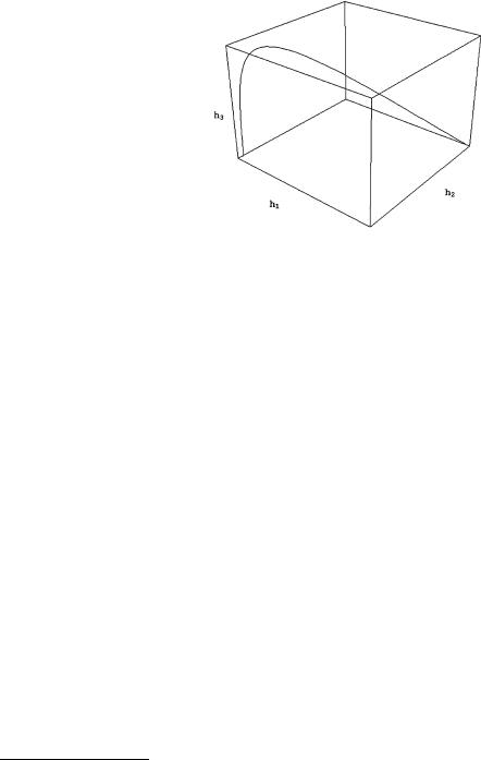
Fig. 5.8 Motion of the fictitious cosmic ball corresponding to the exact Ricci flat metric of Bianchi type II
5.3.4 The Same Billiard with Some Matter Content
We can find an exact solution of the Einstein equations for the above homogeneous but anisotropic Universe if we add some matter content. In order to write the Einstein differential equations in this case, we still need to consider the structure of the stress energy tensor. As usual, in curved indices this is given by:3
T μν = ρU μU ν + p U μU ν − gμν |
(5.3.49) |
where ρ is the energy density, p the pressure and U μ the four-velocity field of the fluid out of which we assume the Universe to be made of. In an isotropic and homogeneous Universe this fluid is assumed to be comoving. Namely, just as we did in the case of stellar equilibrium we assume that the velocity field is orthogonal to the constant time slices of space-time or equivalently that it has vanishing scalar product with all the six space-like Killing vectors:
(−→ −→ |
= |
0 |
(5.3.50) |
U , k ) |
|
In our chosen coordinate system this means U = (1, 0, 0, 0). More intrinsically we can just state that in flat coordinates the stress energy tensor has the following diagonal form:
ρ |
0 |
p(t) |
0 |
0 |
|
|
|
(t) |
0 |
0 |
0 |
|
|
TAB = |
0 |
0 |
p(t) |
0 |
|
(5.3.51) |
|
0 |
0 |
0 |
p(t) |
|
|
|
|
|
|
|
|
|
It is very instructive and of the outmost relevance to calculate the exterior covariant derivative of the above tensor using the spin connection as determined in (5.3.36).
3In the mostly minus conventions we have ds2 = gμν dxμ dxν and gμν U μU ν = 1.

138 5 Cosmology and General Relativity
We get:
T AB = dT AB + ωAF T GB ηF G + ωBF T AF ηF G |
|
|
|
|
|
|
||||||||||||
|
|
E0ρ |
(t) |
E1(p(t |
)+ρ(t))Δ (μ) |
E2(p(t |
)+ρ(t))Λ (μ) |
E3(p(t |
)+ρ(t))Λ (μ) |
|
||||||||
|
|
|
|
|
|
|
||||||||||||
|
|
|
|
|
|
|
2√A(μ)Δ(μ) |
2√A(μ)Λ(μ) |
2√A(μ)Λ(μ) |
|||||||||
|
|
2√A(μ)Δ(μ) |
|
|
|
|
|
|
|
|
|
|
||||||
|
E1 |
(p(t |
)+ρ(t))Δ (μ) |
E1p |
(t) |
0 |
|
|
|
0 |
|
|
||||||
|
|
|
|
|
|
|
||||||||||||
2 |
|
|
)+ρ(t))Λ (μ) |
|
|
|
|
|
|
|
|
|
|
|||||
= E |
(p(t |
0 |
|
E2p |
(t) |
|
|
0 |
|
|
||||||||
|
|
|
|
|
|
|||||||||||||
|
|
2√A(μ)Λ(μ) |
|
|
|
|
|
|
|
|
|
|
||||||
|
|
|
|
|
|
|
|
|
|
|
|
|
|
|
|
|
|
|
|
|
|
+ |
|
|
0 |
|
0 |
|
E p (t) |
|
|||||||
|
2√A(μ)Λ(μ) |
|
|
|||||||||||||||
|
|
|
|
|
|
|
|
3 |
|
|
|
|||||||
E3 |
(p(t) ρ(t))Λ (μ) |
|
|
|
|
|
|
|
|
|
||||||||
|
|
|
|
|
|
|
|
|
|
|
|
|
|
|
|
(5.3.52) |
||
Then we can easily calculate the divergence of the stress-energy tensor, obtaining:
DAT A0 |
= |
|
(p(t) + ρ(t))(Λ(μ)Δ (μ) + 2Δ(μ)Λ (μ)) |
+ |
ρ |
(t) |
= |
0 (5.3.53) |
||
2√ |
|
|
||||||||
|
|
A(μ)Δ(μ)Λ(μ) |
|
|
|
|||||
DAT Ai = 0; (i = 1, . . . , 3) |
|
|
|
|
(5.3.54) |
|||||
Equation (5.3.53) is a conservation equation that can be easily integrated once one knows the equation of state, namely the relation between pressure and energy density:
p = f ( ) |
(5.3.55) |
The equation of state characterizes the type of fluid which is filling up the universe. In the present anisotropic case we are able to find an exact solution of Einstein field equations by using the equation of state of a free scalar field. This is the simple relation:
p = ρ |
(5.3.56) |
To see that this is the equation of state of a free scalar field, it suffices to calculate the stress energy tensor of such a field, assuming that it depends only on time. Anticipating the formula:
Tμν(scal) = |
1 |
∂μφ∂ν φ − |
1 |
gμν ∂ρ φ∂σ φgρσ |
|
2 |
|
4 |
|||
which we derive later in (5.8.4), with a cosmological metric of type ds2 gij dxi dxj , we get:
(5.3.57)
= g00 dt2 +
|
00 = |
4 |
˙ |
; |
|
ij = − 4 |
ij |
|
˙ |
|
T |
|
1 |
φ2 |
|
T |
1 g |
|
g00 |
φ2 |
(5.3.58) |
|
|
|
|
and comparing this with (5.3.49) we identify:
ρ = |
1 |
˙ |
2 |
g |
00 |
; |
p = |
1 |
˙ |
2 |
g |
00 |
(5.3.59) |
4 |
|
|
4 |
|
|
||||||||
|
|
φ |
|
|
|
|
|
|
φ |
|
|
|
|
5.3 Homogeneity Without Isotropy: What Might Happen |
139 |
This implies the equation of state (5.3.56). Substituting such a relation into the conservation equation (5.3.53) we obtain the following differential relation:
ρ(t)Δ (μ) |
+ |
2ρ(t)Λ (μ) |
+ ρ (t) = 0 |
||||
√ |
|
|
√ |
|
|
||
A(μ)Δ(μ) |
A(μ)Λ(μ) |
||||||
which is immediately integrated to:
cost
ρ(t) =
Λ(t)2Δ(t)
If we choose the following linear behavior of the scalar field:
φ = 1 κt
4
where κ is some constant and we choose the following scale factors,
A(t) |
= |
et |
κ32 +ω |
cosh |
tω |
|
||||
|
|
|||||||||
|
2 |
|
||||||||
|
|
e 21 t |
|
cosh |
tω |
|||||
Λ(t) |
= |
κ32 +ω |
||||||||
|
||||||||||
|
2 |
|||||||||
1
Δ(t) = cosh t2ω
by inserting into (5.3.59) we obtain:
|
|
κ2 1 |
|
|
κ2 |
e−t |
|
tω |
|
|
|
|
||||
ρ |
= |
= |
|
κ32 +ω |
sech |
; |
p(t) |
= |
ρ(t) |
|||||||
|
|
|
|
|
||||||||||||
64 A(t) |
64 |
|
||||||||||||||
|
|
2 |
|
|
||||||||||||
(5.3.60)
(5.3.61)
(5.3.62)
(5.3.63)
(5.3.64)
Comparison with (5.3.61) shows that indeed the energy density in (5.3.64) is of the required form and obeys the conservation law, i.e. the field equation of the scalar field. On the other hand calculating the Einstein tensor, namely substituting (5.3.63) into (5.3.40) we get:
|
= |
|
= |
|
= |
|
= |
64 |
|
|
2 |
|
|
G00 |
|
G11 |
|
G22 |
|
G33 |
|
κ2 |
e−t |
κ32 |
+ωsech |
tω |
(5.3.65) |
|
|
|
|
|
|
||||||||
and in this way we verify that Einstein equations are indeed satisfied.
We can now investigate the properties of this solution. First of all we reduce it to the standard form (5.3.43) as we did in the previous case. The procedure is the same, but now the cosmic time τ has a different analytic expression in terms of the original parametric time t . Indeed, substituting the new form of the scale function A(t) as given in (5.3.63) into (5.3.42) we obtain the following definition of the cosmic time:

140 |
5 Cosmology and General Relativity |
Fig. 5.9 The cosmic time τ versus the parameter t for various values of the parameter κ. The bigger κ the thinner the corresponding line. Here κ = 0 is the thickest line. The other two correspond to κ = 1, 2 respectively
|
|
tω |
1 |
κ22 +ω2 |
1 3 |
|
|
κ22 +ω2 |
tω |
/ et (−ω+ |
|
|
)sech( t2ω ) |
||||||
|
|
|
|
2 |
+ω |
||||||||||||||
|
|
2(1+e ) 2 F1(−( |
4 )+ |
|
|
, −( 2 ), 4 + |
|
|
2ω |
, −e ) |
|
|
κ2 |
2 |
|
|
|||
τ (t) |
= |
|
2ω |
|
|
|
|
1+etω |
|
||||||||||
|
|
|
|
|
|
|
|
|
|
|
|
|
|
|
|||||
|
|
|
|
−ω + 2 |
κ2 |
+ ω2 |
|
|
|
|
|||||||||
|
|
|
|
|
|
|
|
|
|
|
|
||||||||
|
|
|
|
|
|
2 |
|
|
|
|
(5.3.66) |
||||||||
|
|
|
|
|
|
|
|
|
|
|
|
|
|
|
|
|
|||
A plot of the function τ (t) for various values of κ (see Fig. 5.9) shows that τ has always the same qualitative behavior. It tends to zero for t → −∞ and it grows exponentially for t → ∞.
Hence we conclude that there is an initial time of this Universe at τ = 0 and we can explore the initial conditions. In a completely different way from the previous vacuum solution, this Universe displays an initial singularity and has a Standard Big Bang behavior. The singularity can be seen in two ways. We can plot the energy density as given in (5.3.64) and realize that for all values of κ = 0 it diverges at the origin of time (see Fig. 5.10).
Alternatively, substituting the scale functions in the expression for the curvature 2-form, we can calculate its limit for t → −∞ and we find that the intrinsic components diverge for all non-vanishing values of κ, while they are finite at κ = 0 which corresponds to the empty universe previously discussed.
Let us now analyze the behavior of the two scale factors Λ(τ ) and Δ(τ ). This is displayed in Fig. 5.11. For late and intermediate times the behavior is just the same as in the vacuum solution with κ = 0, but the novelty is the behavior of Λ at the initial time. Rather than starting from a finite value as in the vacuum solution Λ starts at zero just as . This is the cause of the initial singularity and the Standard Big Bang behavior. Further insight in the behavior of this solution is obtained by considering the evolution plots of the scale factor Λ(τ ) for various values of κ, see Fig. 5.12. We can also look at the behavior of which is plotted in Fig. 5.13.