

150 |
5 Cosmology and General Relativity |
three isotropic, cosmological metrics (5.4.4) admits an alternative description of the Bianchi type, namely:
|
|
|
5 |
3 |
|
|
|
2 |
6 |
|
[ ] = − |
+ |
|
|
|
[ |
] |
|
|||
ds2κ |
dt2 |
a(t)2 |
i 1 |
Ωiκ |
|
(5.4.14) |
||||
|
|
|
=
where the 1-forms Ω[iκ] are left-invariant 1-forms satisfying the Maurer Cartan equations of three different appropriate Lie algebras:
dΩ[iκ] = t[iκ]|j k Ω[jκ] Ω[kκ] |
(5.4.15) |
identified by their structure constants. Explicitly the appropriate algebras are:
type IX |
|
= |
|
|
|
dΩ1 |
= |
Ω2 |
Ω3 |
|
|||
1 |
|
|
3 |
|
1 |
|
2 |
|
|||||
Bianchi |
κ |
|
|
|
dΩ2 |
= Ω |
3 |
Ω |
1 |
|
|||
|
|
|
|
|
|
dΩ |
1 |
= Ω |
1 |
Ω |
3 |
|
|
type V |
|
= − |
|
|
dΩ |
3 |
= |
Ω |
|
Ω |
|
|
|
1 |
|
|
2 |
|
3 |
(5.4.16) |
|||||||
Bianchi |
κ |
|
|
|
dΩ2 |
= Ω |
Ω |
||||||
|
|
|
|
|
|
dΩ |
1 |
= 0 |
|
|
|
|
|
type I |
|
= |
|
|
|
dΩ |
3 |
= |
0 |
|
|
|
|
0 |
|
|
0 |
|
|
|
|
||||||
Bianchi |
κ |
|
|
|
dΩ2 |
= |
|
|
|
|
|||
|
|
|
|
|
|
dΩ |
|
= 0 |
|
|
|
|
|
From this point of view the candidate cosmological metric might have been much more general, i.e.
|
|
ds[2κ] = −dt2 + aij (t)Ω[iκ] Ω[jκ] |
(5.4.17) |
i,j
However such a metric as the above one has only three translational Killing vectors and describes a homogeneous but not isotropic universe. Isotropy follows only from the more restrictive so(3) invariant choice:
aij (t) = a2(t)δij |
(5.4.18) |
5.5Friedman Equations for the Scale Factor and the Equation of State
In order to study the evolution of the cosmic scale factor we need to supplement the conservation equation (5.4.13) with an equation of state for the fluid filling up the universe:
p = f ( ) |
(5.5.1) |
Indeed, upon use of (5.5.1), (5.4.13) reduces to a first order differential equation for the energy density in terms of the scale factor. We shall consider two extreme cases

5.5 Friedman Equations for the Scale Factor and the Equation of State |
151 |
of equations of state: |
|
|
|
p = |
0 |
dust universe |
(5.5.2) |
1 |
radiation universe |
||
|
3 |
|
|
Combining (5.5.2) with (5.4.13) we immediately find: |
|
|||||
|
|
|
|
|
|
|
a3 |
= Cd = const; |
dust universe |
(5.5.3) |
|||
a |
4 |
7r |
= |
; |
|
|
|
= 7 |
|
|
|||
|
|
C |
|
const |
radiation universe |
|
Equations (5.5.3) are conservation laws and their physical interpretation will become clear through our discussion. For the dust case, its meaning should be apparent already at this stage. In a universe uniquely filled with matter, the energy density is, by definition:
matter = |
Total mass of the Universe |
(5.5.4) |
Volume of the Universe |
while, the volume of the Universe at cosmological time t can be identified with:
Volume = a(t)3 |
(5.5.5) |
so that (5.5.3) states that the total mass of the universe is constant in time.
On the other hand for a universe filled with radiation, things are more subtle. The energy of a photon is:
Ephoton = ν |
(5.5.6) |
where ν denotes its frequency. Now assume that the frequency of a photon is redshifted by the expansion according to the law:
νemission = a(tabsorption)
(5.5.7)
νabsorption a(temission)
it follows that the energy density of radiation at any cosmological time is:
|
Number of photons |
1 |
|
||
radiation(t) = |
|
|
× νemission × |
|
(5.5.8) |
Volume of the Universe |
a(t) |
||||
and the second of (5.5.3) is the statement that the total number of photons in the universe is approximately conserved. As we are going to see, the redshift law (5.5.7) is indeed true and a fundamental consequence of general relativity.
A realistic universe is neither pure dust nor pure radiation: it contains both components since there is both granular matter in the form of galaxies and radiation in the form of photons or other ultrarelativistic particles. Their relative contribution to Einstein equations, however, is different at different cosmological times since in an expanding or contracting universe the ratio of the energy densities is:
radiation(t) |
= const × |
1 |
(5.5.9) |
|
|
matter |
a(t) |

152 |
5 Cosmology and General Relativity |
Consequently it makes sense to analyze the solution of the Einstein equations in the two idealized cases where either the radiation or the dust is present. The second solution applies to the present cosmological time when the Universe has already expanded so much that the radiation contribution has become irrelevant, while the first solution applies to early times when radiation was, because of (5.5.9), dominating. Indeed as we are presently going to see from our equations in both cases the behavior of the scale factor a(t) is that of an increasing function of time, at least in a certain initial interval. Later, depending on the value of the curvature κ, the universe can also contract.
5.5.1 Proof of the Cosmological Red-Shift
The overall cosmological red-shift is a consequence of the homogeneity and isotropy of the universe. Let us proof this statement.
Consider the vierbein of a cosmological homogeneous and isotropic space time.
It can be written in the form: |
|
|
E0 = dt; |
Ei = a(t)ei |
(5.5.10) |
where ei denote the vielbein of a three dimensional manifold admitting the transitive action of the symmetry group whose infinitesimal generators are represented by the Killing vectors kI . By definition we have:
|
kei = Wkij ej |
(5.5.11) |
||
where the antisymmetric 3 × 3 |
matrix |
Wkij |
is the so(3)-compensator. Equa- |
|
tion (5.5.11) implies that we also have: |
|
|
|
|
kE0 = |
0; |
kEi |
= Wkij Ej |
(5.5.12) |
The Killing vectors kI have purely space-like components. Correspondingly their squared norm is of the following form:
(k, k) = a2(t) hij ki kj |
(5.5.13) |
||||
|
|
k, |
k |
|
|
|
= |
|
|
! |
|
where k, k! denotes the norm of the same Killing vector in the metric of the constant time sections and it is time independent.
It follows that the ratio of the Killing vector norms at different instant of time equals the corresponding ratio of the scale factors:
|
(k, k)t1 |
a(t1) |
(5.5.14) |
|
|
|
|
||
|
= a(t2) |
|||
(k, k)t2 |
|
|||
5.5 Friedman Equations for the Scale Factor and the Equation of State |
153 |
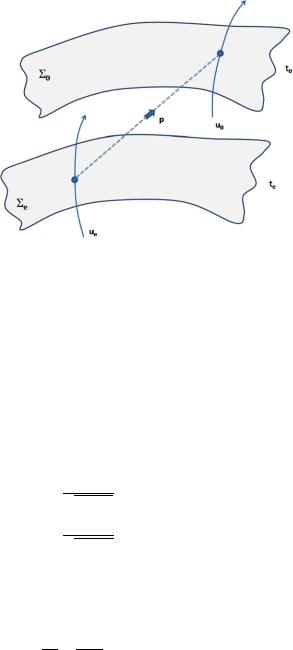
Fig. 5.16 At time te a source having quadri-velocity uμe emits a photon of quadri-momentum kμ that a the later time t0 is absorbed by an observer having quadri-velocity u0. Σe and Σ0 are the constant time slices at the time of emission and of absorption. Both of them are Euclidian three-manifolds admitting the transitive action of the same translation group of isometries
Consider now the situation described in Fig. 5.16. At an early time te a source having quadri-velocity uμe emits a photon of momentum pμ which is later absorbed at time t0 by an observer having four-velocity uμ0 .
By definition the frequency of photon at emission and at absorption are:
ωe = pμueν gμν ; |
ω0 = pμu0ν gμν |
(5.5.15) |
Since the photon is massless we always have that the time and space components of its four-momentum must be equal. On the other hand since the constant time slices of space-time admit the transitive action of a group of isometries, every direction in three space can always be viewed as aligned to a suitable translation space-like Killing vector kν . It follows from this argument that the frequency of the photon at the time of emission and of absorption can also be represented as follows:
= pμkν ωe
(k, k)te
= pμkν ω0
(5.5.16)
(k, k)t0
Next we recall that the scalar product pμkν where pμ is tangent to a geodesic and kν is a Killing vector is constant along the geodesic. This implies that pμkν will be the same at the emission and at the absorption time; consequently, in view of (5.5.14) we obtain:
ωe = a(t0)
(5.5.17)
ω0 a(te)
which is the proof of the cosmological red-shift, already anticipated in previous pages. As we see the key point in the proof is that any direction taken by the threemomentum can be considered aligned to a Killing vector and this is true if our