5.3.3 Einstein Equation and Matter for This Billiard

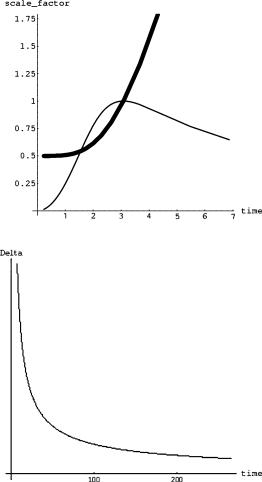
Fig. 5.5 Evolution of the cosmological scale factors

Λ(t) (thick line) and Δ(t)

(thin line) for very early times, when the Universe is very young. Λ starts at a finite value 0.5 and always grows, while starts at zero, grows for some time up to the maximum value 1 and then starts decreasing

Fig. 5.6 Evolution of the cosmological scale factor Δ(t) for late times, when the Universe grows old. tends exponentially to zero

is shown in several graphics. In Fig. 5.5 we see the behavior of the scale factors for very early times.

The early finite behavior of the scale factors has a very important consequence. This space-time has no initial singularity. Indeed for τ → 0 the curvature 2-form is perfectly well behaved and tends to the following finite limit:

its maximum. As we see it rapidly and exponentially tends to zero.

Fig. 5.7 Evolution of the cosmological scale factor Λ(t) for very late times. By now is essentially zero but Λ continues to grow and indefinitely in time with a power law. The graphic plots the logarithm of the scale factor against the logarithm of time and we see an almost perfect straight line

In Fig. 5.7 we see instead the very late time behavior of the scale factor Λ. At asymptotically late times this scale factor grows as a power of time which is slightly smaller than one.

We can summarize by saying that this funny homogeneous but not isotropic Universe, which is empty of matter, has a curious history. It has no initial singularity but it is born finite, small and essentially two-dimensional. It begins to expand and the third dimension starts to develop. It reaches a state when it is effectively threedimensional, although still very small, the two scale factors being of equal size. Then the third dimension rapidly squeezes and the Universe becomes again effectively two dimensional growing monotonously large in the two dimensions in which it was born.

This is an example of the billiard mechanism. The effective dimensions of spacetime change more than once in the course of the cosmic evolution. This is further illustrated in Fig. 5.8 where we show the motion of the fictitious cosmic ball whose coordinates are:

It is evident from the figure that we have two Kasner epochs joined by a smooth bounce. For very early times t → −∞ and for ω > 0 we have