All these features of our toy model apply also to the case of Schwarzschild spacetime once it is extended with the same procedure. The image of the coordinate singularity r = 2m will be a null-like surface, interpreted as event horizon, which can be reached in a finite proper-time but only after an infinite interval of coordinate time. What will be new and of utmost physical interest is precisely the interpretation of the locus r = 2m as an event horizon H which leads to the concept of Black-Hole. Yet this interpretation can be discovered only through the Kruskal extension of Schwarzschild space-time and this latter can be systematically derived via the same algorithm we have applied to the Rindler toy model.

2.2.2 Applying the Same Procedure to the Schwarzschild Metric

We are now ready to analyze the Schwarzschild metric (2.2.1) by means of the tokens illustrated above. The first step consists of reducing it to two-dimensions by fixing the angular coordinates to constant values θ = θ0, φ = φ0. In this way the metric (2.2.1) reduces to:

Next, in the reduced space spanned by the coordinates r and t we look for the nullgeodesics. From the equation:

where we have introduced the so called Regge-Wheeler tortoise coordinate defined by the following indefinite integral:

and the analogue of Fig. 2.4 is now given by Fig. 2.6. Inspection of this picture reveals the same properties we had already observed in the case of the Rindler toy model. What is important to stress in the present model is that each point of the

Fig. 2.6 Null geodesics of the Schwarzschild metric in the r, t plane. The thin curves are incoming (v = const), while the thick ones are outgoing (u = const). Each point in this picture represents a 2-sphere, parameterized by the angles θ0 and φ0. The thick vertical line is the surface r = rS = 2m corresponding to the coordinate singularity. As in the case of the Rindler toy model the null– geodesics incoming from infinity reach the coordinate singularity only at asymptotically late times

t →> +∞. Similarly outgoing null-geodesics were on this surface only at asymptotically early times t → −∞

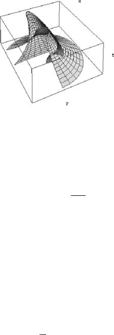
diagram actually represents a 2-sphere parameterized by the two angles θ and φ that we have freezed at the constant values θ0 and φ0. Since we cannot make fourdimensional drawings some pictorial idea of what is going on can be obtained by replacing the 2-sphere with a circle S1 parameterized by the azimuthal angle φ. In this way we obtain a three-dimensional space-time spanned by coordinates t , x = r cos φ, y = r sin φ. In this space the null-geodesics of Fig. 2.6 become twodimensional surfaces. Indeed these null-surfaces are nothing else but the projections θ = θ0 = π/2 of the true null surfaces of the Schwarzschild metric. In Fig. 2.7 we present two examples of such projected null surfaces, one incoming and one outgoing.

Having found the system of incoming and outgoing null-geodesics we go over to point (iii) of our programme and we make a coordinate change from t , r to u, v. By straightforward differentiation of (2.2.20), (2.2.21) we obtain:

so that the reduced Schwarzschild metric (2.2.17) becomes:

Fig. 2.7 An example of two null surfaces generated by null geodesics of the Schwarzschild metric in the r, t plane

Using the definition (2.2.20) of the tortoise coordinate we can also write:

which combined with (2.2.22) yields:

In complete analogy with (2.2.12) we can now introduce the new coordinates:

that play the role of affine parameters along the incoming and outgoing null geodesics.

Then by straightforward differentiation of (2.2.26) the reduced Schwarzschild

where the variable r = r(U, V ) is the function of the independent coordinates U , V implicitly determined by the transcendental equation:

In analogy with our treatment of the Rindler toy model we can make a final coordinate change to new variables X, T related to U , V as in (2.2.14). These, together

with the angular variables θ , φ make up the Kruskal coordinate patch which, putting together all the intermediate steps, is related to the original coordinate patch t , r, θ , φ by the following transition function:

In Kruskal coordinates the Schwarzschild metric (2.2.1) takes the final form:

where the r = r(X, T ) is implicitly determined in terms of X, T by the transcendental equations (2.2.29).

2.2.3 A First Analysis of Kruskal Space-Time

Let us now consider the general properties of the space-time (MKrusk, gKrusk) identified by the metric (2.2.30) and by the implicit definition of the variable r contained in (2.2.29). This analysis is best done by inspection of the two-dimensional diagram displayed in Fig. 2.8. This diagram lies in the plane {X, T }, each of whose points represents a two sphere spanned by the angle-coordinates θ and φ. The first thing to remark concerns the physical range of the coordinates X, T . The Kruskal manifold MKrusk does not coincide with the entire plane, rather it is the infinite portion of the latter comprised between the two branches of the hyperbolic locus:

This is the image in the X, T -plane of the r = 0 locus which is a genuine singularity of both the original Schwarzschild metric and of its Kruskal extension. Indeed from (5.9.6)–(5.9.11) of Volume 1 we know that the intrinsic components of the curvature tensor depend only on r and are singular at r = 0, while they are perfectly regular at r = 2m. Therefore no geodesic can be extended in the X, T plane beyond (2.2.31) which constitutes a boundary of the manifold.

Let us now consider the image of the constant r surfaces. Here we have to distinguish two cases: r > rS or r < rS . We obtain:

Fig. 2.8 A two-dimensional diagram of Kruskal space-time

discussion developed in the next section, the constant r surfaces are space-like outside the sphere of radius rS and time-like inside it. The dividing locus is the pair of straight lines X = ±T which correspond to r = rS and constitute a null-surface, namely one whose normal vector is light-like. This null-surface is the event horizon, a concept whose precise definition needs, in order to be formulated, a careful reconsideration of the notions of Future, Past and Causality in the context of General Relativity. The next two sections pursue such a goal and by their end we will be able to define Black-Holes and their Horizons. Here we note the following. If we solve the geodesic equation for time-like or null-like geodesics with arbitrary initial data inside region II of Fig. 2.8 then the end point of that geodesic is always located on the singular locus T 2 − X2 = −1 and the whole development of the curve occurs inside region II. The formal proof of this statement is involved and it will be overcome by the methods of Sects. 2.3 and 2.4. Yet there is an intuitive argument which provides the correct answer and suffices to clarify the situation. Disregarding the angular variables θ and φ the Kruskal metric (2.2.30) reduces to:

so that it is proportional to two-dimensional Minkowski metric dsMink2 = −dT 2 + dX2 through the positive definite function F (X, T ). In the language of Sect. 2.4

this fact means that, reduced to two-dimensions, Kruskal and Minkowski metrics are conformally equivalent. According to Lemma 2.4.1 proved later on, conformally equivalent metrics share the same light-like geodesics, although the time-like and space-like ones may be different. This means that in two-dimensional Kruskal space-time light travels along straight lines of the form X = ±T + k where k is some constant. This is the same statement as saying that at any point p of the {X, T } plane the tangent vector to any curve is time-like or light-like and oriented to the future if