5.6.1 Particle Horizon

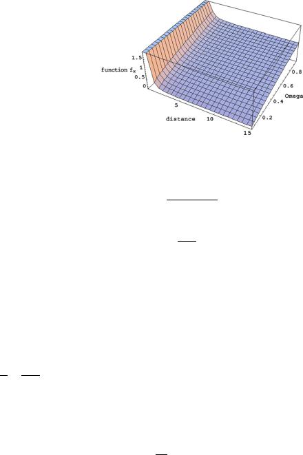
Fig. 5.22 Plot of the function f−1(d0, Ω0) showing that it is bounded and of order unity

where the functions fκ (d0, Ω0) depend on the sign of the spatial curvature and are listed below

The relevant point of the above calculation is that the three functions fκ (d0, Ω0) are all bounded and of order unity in the range where they are physically significant. For the case of the spatially flat Universe (κ = 0) this is obvious. In the case of an open Universe κ = −1 the expansion is indefinite and there is no limit to the distance d0 that we can consider. On the other hand the cosmological parameter is defined only in the range 0 < Ω0 < 1. Therefore we have to restrict our attention to the open strip (]0, ∞[) × (]0, 1[) R2. There the function f−1(d0, Ω0) is bounded and takes values in the interval [0, 2]. Its very smooth plot is shown in Fig. 5.22. In the case of a closed Universe (κ = 1) the cosmological parameter is bounded only from below (Ω0 > 1), but there is always a maximal distance that we can explore

a corresponding to the absolute maximum reached by the scale factor

a0

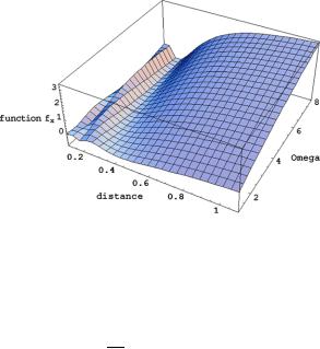
during the whole history of such a Universe. The plot of the function f1(d0, Ω0) in the physically available range is slightly more structured yet it is also bounded and of order unity as it is shown in Fig. 5.23. The outshot of such a discussion is that in a matter dominated Universe the particle horizon is finite and its scale is fixed by the inverse of the Hubble constant:

Completely different is the conclusion one reaches in an exponentially expanding Universe dominated by vacuum energy. Suppose we sit at time t0 and suppose that

Fig. 5.23 Plot of the function f1(d0, Ω0) showing that it is bounded and of order unity in the physically available range

in our past the Universe was expanding according to the law dictated by w = −1. To simplify matters let us also assume that we deal with a spatially flat Universe κ = 0. In that case the Hubble function is actually a Hubble constant H0 and from the integral in (5.6.28) we obtain:

In the limit ai → 0 we see that dp → ∞, in other words if the exponential expansion phase started at the very beginning of the Universe, there is no particle horizon and the distance that can be seen at any later moment of the exponential expansion extends to the whole physical space. This has a very important consequence which is the basic motivation to consider inflation. What we can see from the past is what can influence our present, namely what is in causal contact with us. Therefore we can conclude that at the end of an exponential expansion, if that expansion started early enough (ai 0), the entire resulting Universe originated from a single causally connected region. If the subsequent expansion of the Universe proceeds through a matter dominated regime, from the perspective of an observer living in that age, the same Universe appears instead to be made of a plethora of causally disconnected regions. This observation will play a fundamental role in understanding why the inflationary scenario solves the puzzles of the Standard Cosmological Model in a robust way.

5.6.2 Event Horizon

The event-horizon is the complement of the particle horizon. By definition the eventhorizon is the boundary of the space-time region from which no signal will ever be received by an observer in its future. According to this definition the events inside the event-horizon are characterized by radial coordinates χ larger than the following

where η is the conformal time when the considered observer lives while ηend is the conformal date of death of the Universe. Therefore, in full analogy to our treatment of the particle horizon, the size of the event horizon at current cosmic time t0 is determined by:

Hence for a matter dominated Universe we obtain:

In both cases of an open and a flat universe the above integral diverges for aend → ∞ and therefore there is no event horizon. Different is the case of a matter dominated, closed Universe. There the scale factor reaches a maximum and then decreases to zero at the Big Crunch. Recalling (5.5.22)–(5.5.23) we see that in the case of this universe the conformal time is bounded by ηend = 2π , so that we obtain:

where amax is the maximal value of the scale factor attained in the history of the closed universe, which after that decreases until it vanishes again at the Big Crunch. The last identity in (5.6.37) is a consequence of the periodicity of trigonometric functions, sin2(2π − η) = sin2(η), which implies a remarkable consequence: in closed universes the event and the particle horizons exactly coincide. In the first expansion phase the event horizon grows along with the scale factor but while the expansion slows down, it reaches a maximum corresponding to 23 amax and then starts decreasing again until it shrinks to zero at the same time when the Universe attains its maximal extension. After that, while the Universe begins to contract, the event horizon grows once more and attains again the same maximum 23 amax. Then it shrinks along with the Universe and becomes zero at the Big Crunch. The plot of the event/particle horizon and of the scale factor are compared in Fig. 5.24.

Hence the visible portion of a closed Universe enlarges and shrinks with a different periodicity with respect to the expansion scale-time. This leads to the surprising result that the visible portion of the Universe shrinks almost to zero when it attains its maximal extension.

Something quite different happens in an exponentially expanding universe. For simplicity focusing once again on the case of a spatially flat de Sitter space, we

Fig. 5.24 Plot of the scale factor and of the event/particle horizon in a spatially positively curved, matter dominated universe. In both pictures the thin line corresponds to the scale factor, while the thicker one corresponds to the event/particle-horizon. In the

first picture both a and de/p are plotted against the conformal time η, while in the second they are plotted against the physical time t

calculate there the event horizon:

where we have made use of (5.5.54). Hence while the Universe undergoes an exponential expansion the event horizon remains constant and its size is fixed by the inverse Hubble constant. The set of events causally disconnected from the observer fills a region which becomes bigger and bigger as time goes on. This elementary fact has striking implications within the inflationary scenario.

Consider a quantum particle emitted in some physical process at some instant of time during an exponential expansion phase of the Universe. Suppose that its wave-length at the emission time is λe < H0−1, which we describe by saying that it is inside the Hubble radius. Stretched by the cosmological red-shift, at a time t defined by λe = H0−1 that wave-length exits the Hubble horizon and becomes larger than the current event horizon. After that time all physical quantities associated with such a wave-length freeze out, since no physical process can any more alter them. If the exponential expansion phase is followed by another one where the Universe continues to expand according to a power-like law, then the Hubble scale H −1(t) will grow once again and the considered primordial wave-length might reenter, at a later time, the Hubble radius. At that moment the physical quantities associated with it will be transformed by interactions with the other components of the post-inflationary Universe and their state at the present time will depend also on the post-inflationary evolution. At distances larger than the Hubble radius, we see instead faithful images of the remote age associated with the conjectured exponential expansion.