


5.8 Cosmic Evolution with a Scalar Field: The Basis for Inflation |
177 |
This observation is the corner-stones of the inflationary scenario.
Imagine that, at some very ancient instant of time ti , a small region of the spacetime manifold, containing matter and energy of various types, begins to inflate since, over that region, the scalar field ϕ is approximately constant and equal to the critical value ϕ0. The approximate behavior of this expanding space-time bubble will be the same as that of a region of de Sitter space. At the beginning ti , the spatial curvature of the bubble might have been positive, negative or null, yet at a sufficiently later time tend, the effective metric of the bubble will be that of a spatially flat deSitter manifold dsdS2 0 . Suppose now that at t = tend the scalar field, which was so far approximately constant, begins to evolve more rapidly and the kinetic energy ϕ˙2 starts dominating over the potential energy V (ϕ) which has in the meantime decreased. According to Friedman equations the acceleration parameter changes sign, the expansion rate decreases and, in a finite time, the behavior of the scale factor approaches that of a Universe filled with ordinary baryonic matter and radiation. Yet, the considered space-time bubble is spatially-flat as a result of the inflation which has occurred in the previous phase. This fundamental property of an inflationary phase in the history of the Universe is the most relevant feature of the inflationary scenario. It explains in a natural way and without ad hoc fine tuning why our Universe is spatially flat as it happens to reveal itself through experimental observations.
As we plan to analyze more explicitly in the sequel, the inflationary phase explains also why the observable Universe is homogeneous to very high accuracy over regions that are causally disconnected at the present time.
5.8.2 Slow-Rolling Approximate Solutions
In view of the qualitative considerations discussed above, let us now consider approximate solutions of (5.8.7), (5.8.8), (5.8.10) corresponding to a slow-roll phase. This latter is defined by the following two conditions:
1 |
ϕ˙2 ' V (ϕ) |
|
|
|
(5.8.16) |
|
2 |
|
|
|
|||
|
¨ ' |
˙ + |
V (ϕ) |
0 |
(5.8.17) |
|
|
ϕ |
3H ϕ |
|
|||
whose physical interpretation is quite transparent, the former requiring that the kinetic energy of the scalar field should be negligible with respect to the potential energy, the latter requiring that the acceleration in the evolution of ϕ should also be small with respect to the velocity.
In order to discuss the existence and the properties of such a regime, it is convenient to manipulate a little bit the evolution equations (5.8.7), (5.8.8), (5.8.10) casting them in a more manageable form. First of all it is convenient to introduce rescaled variables so as to get rid of all the constants. Introducing the Planck mass:
1 |
|
mP = √2π G |
(5.8.18) |

178 |
|
|
|
|
|
|
|
|
|
|
|
|
|
|
5 Cosmology and General Relativity |
|||||||
we set: |
|
|
V (ϕ) = mP2 W |
mP |
= mP W (φ) |
|
|
(5.8.19) |
||||||||||||||
ϕ = mP φ; |
|
|
|
|
||||||||||||||||||
|
|
|
|
|
|
|
|
|
|
|
|
|
|
|
ϕ |
|
|
|
|
|
|
|
|
|
|
|
|
|
|
|
|
|
|
|
|
|
|
|
|
|
a |
= |
˙ |
+ |
H 2 we ob- |
Substituting in (5.8.7), (5.8.8), (5.8.10) and using the identity a¨ |
|
H |
|
|||||||||||||||||||
tain: |
|
|
|
|
|
|
|
|
|
|
|
|
|
|
|
|
|
|
|
|
|
|
|
|
|
|
|
2 |
|
1 |
φ2 |
|
|
2 |
W |
|
|
|
|
|
|
(5.8.20) |
|||
|
|
|
|
H |
|
= 3 |
+ |
3 |
|
|
|
|
|
|
||||||||
|
|
˙ |
+ |
|
|
˙ |
|
|
|
|
|
|
|
|
|
|
||||||
|
|
|
|
= − |
3 |
˙ |
+ |
|
3 |
|
|
|
|
|
|
|
||||||
|
H |
|
H |
2 |
|
|
|
2 |
φ2 |
|
|
|
2 W |
|
|
|
|
|
(5.8.21) |
|||
|
|
|
= ¨ |
|
|
|
˙ |
|
|
|
|
|
||||||||||
|
|
|
|
|
0 |
|
+ |
|
|
+ |
W |
|
|
|
|
(5.8.22) |
||||||
|
|
|
|
|
φ |
|
|
|
3H φ |
|
|
|
|
|
||||||||
where we have already set |
κ |
= 0 in view of the discussion of |
the previous section. |
|||||||||||||||||||
|
|
5 |
|
|
|
|||||||||||||||||
This shows that our system of equations is actually a (redundant ) differential system for the scalar field φ(t) and the Hubble function H (t). The de Sitter solution is nothing else but the constant solution φ = φ0, H = H0, which requires that φ0 should sit at an extremum of the potential V (φ0) = 0. The main idea of the slow rolling consists of considering the evolution of the two functions H (t) and φ(t) starting from an initial configuration which is very close to de Sitter one. At t = ti the scalar field does not sit at an extremum of the potential, yet not too far from
it (V (φi ) |
≈ |
|
|
|
˙ |
≈ |
small and small is the initial |
|
small), its initial velocity is small φi |
|
|||||
derivative of the Hubble function |
˙ |
i ) small. The latter condition is not inde- |
|||||
|
|
|
H (t |
of ≈ |
|
|
|
pendent rather it is just a consequence |
|
|
φ |
||||
the smallness of ˙i . Indeed from (5.8.22), |
|||||||
it follows: |
|
|
˙ |
= − ˙ |
|
|
|
|
|
|
|
(5.8.23) |
|||
|
|
|
H |
|
φ2 |
|
|
Obviously such initial conditions can always be postulated, yet the question is whether they can be maintained throughout evolution at least for a certain nonnegligible period of time during which the Universe will experience an almost exponential expansion like if it were a true de Sitter space. The answer to such a question depends on the properties of the scalar potential. Several types of potentials have been used in the explicit modeling of Inflation, trying also to relate them with the fundamental theories of Particle Interactions, in particular with the scenario of symmetry breaking and with the Higgs mechanism. Indeed it has been conjectured that the inflaton, i.e. the scalar field responsible for the primeval exponential growth of the Universe should be a condensate of the scalar degrees of freedom available in the fundamental unified theory of all interactions which describes Physics at the Planck scale and hence at the Big Bang. Inspired by this natural point of view, in more recent time attentive consideration has been given to the many field potentials V (φ1 . . . φn) which arise in supergravity theory, induced by the brane-superstring
5Any one of the three equations is actually a consequence of the other two as a legacy of the Bianchi identities which constrain Einstein equations.
5.8 Cosmic Evolution with a Scalar Field: The Basis for Inflation |
179 |
scenarios. We shall not enter the fine structure of inflation modeling, which is still in lively evolution, since the most relevant and appealing feature of the inflationary scenario is precisely its robustness. The main physical mechanism and the essence of its predictions are largely independent from the detailed structure of the utilized potential, provided it is sufficiently smooth and reasonable. What this concretely means we shall presently show. Therefore, for the sake of simplicity we focus on the most widely utilized type of potentials that are the polynomial ones, in particular the following one
W (φ) = −μφα + λφ2α + |
ν |
(5.8.24) |
4λ |
which for various values of the parameters λ, μ, ν captures the main features of three distinct well-known modelings of inflation.
(a)For μ = ν = 0 we have the so named large field modeling of inflation. The potential has just a minimum at φ = 0 and slow roll, as we shall prove below is obtained by starting at some sufficiently high value of φi .
(b)For μ = 0 we have the so named small field modeling. The potential has just a
maximum at φ = 0 and a minimum at φ = ( 4νλ2 )1/2α . Slow rolling is obtained by starting at small values φi of the field near the unstable maximum.
(c)For ν = μ2 the potential becomes:
|
= |
|
|
− |
2√λ |
2 |
|
|
W (φ) |
√λφ |
|
μ |
|
(5.8.25) |
|||
which again has a maximum and a minimum and corresponds to the sort of potentials appearing in the symmetry breaking scenarios. In this case, as in the previous ones, slow rolling is obtained by starting at small values φi of the field, near the maximum.
Independently from the explicit form of the potential let us consider the consistency conditions imposed on it by the assuming the existence of a slow rolling phase. From the exact result (5.8.23) we know that if the scalar field has a slow roll, even slower will be the change of the Hubble function. Consider next the slow-roll condition (5.8.17) from which we work out
φ |
− |
W |
(5.8.26) |
|
3H |
||||
˙ |
and insert this result into the first condition (5.8.16). We obtain:
1 (W |
)2 |
|
|
|
1 |
W |
2 |
|
||||
|
|
|
|
' W |
|
εW (φ) ≡ |
|
|
|
|
' 1 |
(5.8.27) |
6 |
W |
|
6 |
W |
||||||||
We see that a necessary condition for slow roll corresponds to the smallness of a certain function εW (φ) of the scalar field, defined in (5.8.27) and completely determined by the potential. This condition is not the only one. Taking a further derivative
180 |
5 Cosmology and General Relativity |
of condition (5.8.16) we get:
3φH |
+ |
3φH |
W |
φ |
|
0 |
φ |
− |
W |
W |
+ |
W |
H |
(5.8.28) |
|
9H 2 |
3H 2 |
||||||||||||||
¨ |
˙ ˙ + |
|
˙ |
|
¨ |
|
˙ |
|
where ˙ has been eliminated by means of the slow-roll condition (5.8.26). From the |
||||||||||
φ |
' |
|
|
|
|
|
|
|
|
|
¨ |
W |
, using (5.8.28) and eliminating H 2 by means of (5.8.16) and H |
||||||||
condition φ |
|
|||||||||
first by means of the exact result (5.8.23) then by means of (5.8.16) we get: |
|
|||||||||
|
|
|
|
1 W |
1 |
|
|
|||
|
|
|
|
|
|
|
+ |
|
εW ' 1 |
(5.8.29) |
|
|
|
|
6 W |
3H |
|||||
Since we already know that εW ' 1 and 3H > 1, it follows that:
ηW (φ) ≡ |
1 W |
' 1 |
(5.8.30) |
6 W |
Hence we conclude that the smallness of the two functions εW (φ) and ηW (φ) is a necessary condition for slow-rolling.
In the case of the potential (5.8.25), the explicit form of the two slow roll index functions is:
ε |
W |
(φ) |
= |
|
8α2λ2φ2α−2(μ − 2λφα )2 |
|
(5.8.31) |
|
3(4λ(λφα − μ)φα + ν)2 |
||||||||
|
|
|
|
|||||
η |
W |
(φ) |
= |
|
2αλφα−2(2(2α − 1)λφα − αμ + μ) |
(5.8.32) |
||
3(4λ(λφα − μ)φα + ν) |
||||||||
|
|
|
|
|||||
which, in the two particular subcases that we respectively named large field and symmetry breaking, reduces to:
large field εW = 32φα2 |
|
|
|
|||
|
|
|
2 |
|
|
|
|
ηW |
= |
α(2α−2 1) |
|
|
(5.8.33) |
|
|
8α2λ2φ2α−2 |
||||
|
|
|
3φ |
|
|
|
|
η |
= |
|
|
|
|
2αλφα−2 |
(2(2α−1)λφα −αμ+μ) |
|
||||
symm. break. |
εW |
3(μ−2λφα )2 |
|
|||
W = |
|
3(μ−2λφα )2 |
|
|||
The rationale for the given names becomes now clear. In the large field case the conditions εV ' 1 and ηV ' 1 translate into:
|
3 |
|
− |
1) < |
3 |
|
' |
|
|
1 |
α(2α |
|
1 |
2α2 |
|
φ |
(5.8.34) |
||
|
|
|
|
while in the symmetry breaking case the same conditions have two solutions, either
μ
φ &
2λ
1
α
(5.8.35)
5.8 Cosmic Evolution with a Scalar Field: The Basis for Inflation |
181 |
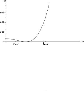
Fig. 5.25 |
Picture of the potential (5.8.24) for an explicit |
choice of the parameters that cor- |
|||||||
responds |
to the |
symmetry breaking case: λ = 1, μ = 16, |
ν = 256. In this case we obtain: |
||||||
W (φ) = (−8 + |
φ |
2 |
) |
2 |
|
√ |
|
|
|
|
|
. Such a function has a maximum at φ = 0 and a minimum at φ = 2 2. |
|||||||
On both sides of the maximum we have values named φend , whose precise definition is explained in the text, at which inflation ends for a slow rolling starting on the left or on the right of the minimum
or
μ
φ '
2λ
1
α
(5.8.36)
Hence in the large field case the slow-roll conditions are realized when the field is sufficiently large, while in the symmetry breaking case they are realized when it is either sufficiently large or sufficiently small as to be reasonably distant from the minimum of the potential where both indices εW (φ) and ηW (φ) develop a pole (see Fig. 5.26). This means that in the cosmic evolution which starts from initial conditions corresponding to slow-roll we will have slow-rolling and inflation while the field φ remains in the region where the two indices are small. Inflation will end as soon as these indices become of finite size and conventionally we can fix the end of inflation at:
φend : εW (φend) = 1 |
|
|
|
|
|
(5.8.37) |
|||
For the large field case we can give the general formula: |
|
|
|
|
|
||||
|
|
|
|
|
|
|
|
|
|
large field scenario |
: |
φend |
= |
|
2 |
|
α |
(5.8.38) |
|
3 |
|
||||||||
|
|
|
|
|
|
||||
while in the symmetry breaking case a general solution of the implicit equation (5.8.37) cannot be written for all values of the power α and they have to be worked out case by case. Relying on these general observations we can now illustrate the mechanism of inflation by considering a specific case of the symmetry breaking scenario whose corresponding differential equations we will solve numerically. The qualitative picture is presented in Fig. 5.27.
We have an attractive mechanical analogy with a ball that is rolling down a hill towards the bottom of a valley that corresponds to the minimal of the potential. At the beginning the ball rolls slowly and its kinetic energy is negligible with respect
182 5 Cosmology and General Relativity
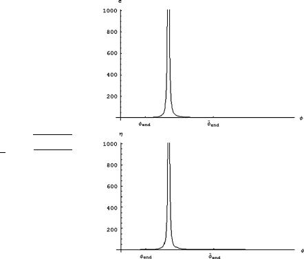
Fig. 5.26 In this picture we present the plot of the slow roll indices εW (φ) and ηW (φ) for the example of symmetry breaking potential presented in Fig. 5.25 corresponding to (5.8.24) with parameters:
λ = 1, μ = 16, ν = 256. In this case we obtain:
εW (φ) = |
8φ2 |
||||
|
and |
||||
3(φ2−2 8)2 |
|||||
η |
W |
(φ) |
= |
2(3φ −8) . |
|
|
|
3(φ2−8)2 |
|||
Correspondingly we have two |
|
solutions for the end of |
|
inflation field value, namely |
|
φend = 2 |
31 (7 − √13) and |
φend = 2 |
31 (7 + √13) which |
respectively sit before and after the minimum of the potential where the indices develop a pole
to the potential energy that drives an exponential growth of the scale factor. This is the inflation phase during which, dominated by vacuum energy, the Universe is very cold. Notwithstanding the slow rolling the ball goes down and it reaches the point where the slow rolling conditions cease to be valid. This is the end of inflation. After that the ball continues its descent, accelerating its motion while the growth of the scale factor experiences a rapid change of gear from an exponential to a power law one. Reaching the minimum the scalar field oscillates around it rapidly but with damped amplitude until it definitely sits down in the stable position. In order to verify the above qualitative description numerically it is convenient to rewrite the evolution equations (5.8.22) as a pair of second order coupled differential equations which we achieve as follows:
2 a(t) + a(t) − |
|
|
= |
|
|
||||||||||||
|
1 |
|
a(t¨ ) |
|
|
a(t˙ ) |
|
|
|
W φ(t) |
|
0 |
(5.8.39) |
||||
¨ |
|
|
˙ |
|
|
= |
|||||||||||
|
+ |
|
a(t) |
+ |
|
|
|
|
|
||||||||
φ(t) |
|
|
|
3 |
|
a(t˙ ) |
|
φ(t) |
|
W |
φ(t) |
|
0 |
(5.8.40) |
|||
|
|
|
|
|
|
|
|
||||||||||
Starting from (5.8.25), if we choose the power α = 2 and the parameters λ = 1, μ = 16, ν = 256, which is the choice graphically displayed in Fig. 5.25 and already
5.8 Cosmic Evolution with a Scalar Field: The Basis for Inflation |
183 |
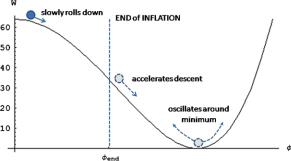
Fig. 5.27 The initial condition for cosmic evolution corresponds to a situation where the scalar field is at some value not too far from a maximum of the potential. Then the scalar starts rolling down from the hill towards the minimum. At the beginning the condition of slow rolling are satisfied. The scalar changes slowly while the scale factor increases almost exponentially. Going downhill the scalar reaches such a value where the slow-roll parameter εW becomes of order unity. There inflation ends since the kinetic energy of φ becomes comparable to its potential energy. The exponential growth of the scalar field ceases while the field φ accelerates towards the minimum. Around the minimum the scalar oscillates rapidly and its energy is dispersed by reheating the Universe
used also in the other plots, then the potential becomes:
W (φ) = φ2 − 8 2; W (φ) = 4φ φ2 − 8 |
(5.8.41) |
Replacing such explicit functions in (5.8.40), we can solve them numerically if we provide initial conditions at the initial time ti which we can conventionally fix at zero ti = 0. This means that we have to give the following data:
a(0) |
= |
a |
0; |
˙ |
= ˙ |
0; |
φ(0) |
= |
φ |
0; |
˙ 0 |
= ˙0 |
(5.8.42) |
|
|
a(0) |
a |
|
|
|
φ( ) |
φ |
It is important to stress that inflation will take place if and only if such initial conditions are given in such a way as to be consistent with the slow roll. This means first of all that φ0 must be chosen in the region where εW (φ0) ' 1 and ηW (φ0) ' 1.
Furthermore, once φ0 has been chosen, |
˙ |
and |
˙ |
0 must be chosen in such a way |
|||||||||
a0 |
|||||||||||||
|
|
|
|
|
|
|
|
|
|
|
φ |
|
|
that: |
|
|
|
|
|
|
|
|
|
|
|
|
|
93 |
a˙0 |
φ0 |
+ |
W |
(φ0)9 |
' |
1 |
||||||
|
|
||||||||||||
9 |
|
a0 |
2 |
|
|
|
9 |
1 |
|||||
9a˙ |
0 |
|
|
|
2 W (φ )9 |
|
|||||||
9 |
|
|
|
|
|
|
|
|
|
|
9 |
|
(5.8.43) |
9 |
|
|
|
− |
|
|
0 |
9 |
' |
|
|||
a |
0 |
3 |
|
|
|||||||||
9 |
|
|
|
|
|
|
|
9 |
|
||||
9 |
|
|
|
|
|
|
|
|
|
|
9 |
|
|
9 |
|
|
|
|
|
|
|
|
|
|
9 |
|
|
In this way we begin with slow roll and the slow roll phase hopefully will last for a sufficiently long interval of time as to allow the expansion of the scale factor by several order of magnitudes. In Fig. 5.28 we present the numerical solution of
184 |
5 Cosmology and General Relativity |
Fig. 5.28 Overall plot of the solution of the coupled differential equations (5.8.40) for the scale factor a(t) and the scalar field φ(t) clearly displaying an early phase of slow rolling. The potential is that given in (5.8.41) and the initial conditions are those displayed in (5.8.44). In the inflation phase, lasting approximately in the interval of time from t = 0 to t = 2.5, the scale factor increases of almost 14 orders of magnitudes. As discussed in the text, this is not yet the sufficient amount of inflation to solve the horizon problem of cosmology. For that we need about 60 order of magnitudes (e-foldings)
(5.8.40) with the potential (5.8.41) and the following initial conditions:
φ0 |
|
0.1 |
|
φ0 |
φ |
|
|
|
|
|
|
1 |
|
|
W |
(φ0) |
|
0.133333 |
|
|
|
≡ − a0 |
|
|
|
|
|
|
|||||||||||
|
= |
|
|
; |
˙ |
= ˙0 |
|
32 W (φ0) |
|
|
= |
(5.8.44) |
|||||||
a0 |
= |
1 |
; |
|
a0 |
a0 |
≡ |
a0 |
|
2 |
W (φ0) |
= |
7.99 |
|
|
||||
|
3 |
|
|
||||||||||||||||
|
|
|
˙ |
= ˙ |
|
|
|
|
|
|
|
|
|||||||
which saturate the bounds (5.8.43). Clearly we have an inflation phase which lasts up to φend and inflates the Universe by about 14 orders of magnitudes. In Fig. 5.29 we present an enlargement of the same plot for later times, namely for t > 3. It is evident that the exponential expansion of the scale factor is now replaced by a power law growth which is weaker than linear as in a matter dominated Universe where a t2/3. At the same time the scalar field displays a damped rapid oscillation around the value corresponding to a minimum of the potential.
The existence of a good bona-fide slow roll phase in the numerical solution corresponding to the chosen initial conditions is best certified by the plot of the function
φ(t) |
|
3H (t) ˙ |
|
f (t) ≡ − W (φ(t)) |
(5.8.45) |

5.8 Cosmic Evolution with a Scalar Field: The Basis for Inflation |
185 |
Fig. 5.29 After the end of inflation the growth of the scalar factor becomes of power type a tp with
p < 1. At the same time the scalar field undergoes rapid damped oscillations around the value φmin corresponding to a minimum of the potential
evaluated on the solution. This plot is presented in the first picture of Fig. 5.30. As we see, f (t) is essentially constant and equal to one in the whole interval of time from t = 0 to t = 2.3. This is the epoch of inflation. After that f (t) rapidly diverges signaling the end of the slow roll.
The important question which so far has no analytic answer is the following one.
How large is the domain of initial conditions around the critical values ˙ and ˙ for a0 φ0
which there is a slow roll phase? The relevance of this question can be appreciated a posteriori considering numerical solutions with initial conditions:
|
φ(0) |
= |
φ |
+ |
φ |
; |
˙ |
= ˙ |
|
+ |
˙ |
|
|
|
˙ |
|
˙0 |
˙ |
|
(5.8.46) |
|||||||
|
|
|
|
|
a(0) |
a0 |
|
a |
|||||
Experimentally for |
˙ |
and |
˙ |
not too large we find solutions that are very sim- |
|||||||||
|
φ |
|
|
a |
|
|
|
|
|
|
|
|
|
ilar to the solution in Fig. 5.28. Yet for somewhat larger deviations in the initial conditions the qualitative picture of slow roll and inflation is completely destroyed.
For instance if we choose |
˙ = |
100 and |
˙ |
= |
1500 we obtain a solution where |
a |
|
||||
|
|
|
φ |
|
|
there is essentially no period of exponential growth of the scale factor (the Hubble function is never approximately constant) and the scalar field almost immediately oscillates. The essential absence of a slow rolling phase is certified by the plot of the function f (t) which for such a solution is displayed in the second picture of Fig. 5.30.
It is evident that a decisive progress in the mathematical foundations of the inflationary scenario and on its robustness will come only from a proper definition of the domain of attraction of the slow rolling regime. Indeed it is important to establish how generic are the initial conditions that lead to inflation and therefore produce a flat, homogeneous universe like ours.