- •Preface
- •Acknowledgements
- •Contents
- •2.1 Introduction and a Short History of Black Holes
- •2.2 The Kruskal Extension of Schwarzschild Space-Time
- •2.2.1 Analysis of the Rindler Space-Time
- •2.2.2 Applying the Same Procedure to the Schwarzschild Metric
- •2.2.3 A First Analysis of Kruskal Space-Time
- •2.3 Basic Concepts about Future, Past and Causality
- •2.3.1 The Light-Cone
- •2.3.2 Future and Past of Events and Regions
- •Achronal Sets
- •Time-Orientability
- •Domains of Dependence
- •Cauchy surfaces
- •2.4.1 Conformal Mapping of Minkowski Space into the Einstein Static Universe
- •2.4.2 Asymptotic Flatness
- •2.5 The Causal Boundary of Kruskal Space-Time
- •References
- •3.1 Introduction
- •3.2 The Kerr-Newman Metric
- •3.2.1 Riemann and Ricci Curvatures of the Kerr-Newman Metric
- •3.3 The Static Limit in Kerr-Newman Space-Time
- •Static Observers
- •3.4 The Horizon and the Ergosphere
- •The Horizon Area
- •3.5 Geodesics of the Kerr Metric
- •3.5.2 The Hamilton-Jacobi Equation and the Carter Constant
- •3.5.3 Reduction to First Order Equations
- •3.5.4 The Exact Solution of the Schwarzschild Orbit Equation as an Application
- •3.5.5 About Explicit Kerr Geodesics
- •3.6 The Kerr Black Hole and the Laws of Thermodynamics
- •3.6.1 The Penrose Mechanism
- •3.6.2 The Bekenstein Hawking Entropy and Hawking Radiation
- •References
- •4.1 Historical Introduction to Modern Cosmology
- •4.2 The Universe Is a Dynamical System
- •4.3 Expansion of the Universe
- •4.3.1 Why the Night is Dark and Olbers Paradox
- •4.3.2 Hubble, the Galaxies and the Great Debate
- •4.3.4 The Big Bang
- •4.4 The Cosmological Principle
- •4.5 The Cosmic Background Radiation
- •4.6 The New Scenario of the Inflationary Universe
- •4.7 The End of the Second Millennium and the Dawn of the Third Bring Great News in Cosmology
- •References
- •5.1 Introduction
- •5.2 Mathematical Interlude: Isometries and the Geometry of Coset Manifolds
- •5.2.1 Isometries and Killing Vector Fields
- •5.2.2 Coset Manifolds
- •5.2.3 The Geometry of Coset Manifolds
- •5.2.3.1 Infinitesimal Transformations and Killing Vectors
- •5.2.3.2 Vielbeins, Connections and Metrics on G/H
- •5.2.3.3 Lie Derivatives
- •5.2.3.4 Invariant Metrics on Coset Manifolds
- •5.2.3.5 For Spheres and Pseudo-Spheres
- •5.3 Homogeneity Without Isotropy: What Might Happen
- •5.3.1 Bianchi Spaces and Kasner Metrics
- •5.3.1.1 Bianchi Type I and Kasner Metrics
- •5.3.2.1 A Ricci Flat Bianchi II Metric
- •5.3.3 Einstein Equation and Matter for This Billiard
- •5.3.4 The Same Billiard with Some Matter Content
- •5.3.5 Three-Space Geometry of This Toy Model
- •5.4 The Standard Cosmological Model: Isotropic and Homogeneous Metrics
- •5.4.1 Viewing the Coset Manifolds as Group Manifolds
- •5.5 Friedman Equations for the Scale Factor and the Equation of State
- •5.5.1 Proof of the Cosmological Red-Shift
- •5.5.2 Solution of the Cosmological Differential Equations for Dust and Radiation Without a Cosmological Constant
- •5.5.3 Embedding Cosmologies into de Sitter Space
- •5.6 General Consequences of Friedman Equations
- •5.6.1 Particle Horizon
- •5.6.2 Event Horizon
- •5.6.3 Red-Shift Distances
- •5.7 Conceptual Problems of the Standard Cosmological Model
- •5.8 Cosmic Evolution with a Scalar Field: The Basis for Inflation
- •5.8.1 de Sitter Solution
- •5.8.2 Slow-Rolling Approximate Solutions
- •5.8.2.1 Number of e-Folds
- •5.9 Primordial Perturbations of the Cosmological Metric and of the Inflaton
- •5.9.1 The Conformal Frame
- •5.9.2 Deriving the Equations for the Perturbation
- •5.9.2.1 Meaning of the Propagation Equation
- •5.9.2.2 Evaluation of the Effective Mass Term in the Slow Roll Approximation
- •5.9.2.3 Derivation of the Propagation Equation
- •5.9.3 Quantization of the Scalar Degree of Freedom
- •5.9.4 Calculation of the Power Spectrum in the Two Regimes
- •5.9.4.1 Short Wave-Lengths
- •5.9.4.2 Long Wave-Lengths
- •5.9.4.3 Gluing the Long and Short Wave-Length Solutions Together
- •5.9.4.4 The Spectral Index
- •5.10 The Anisotropies of the Cosmic Microwave Background
- •5.10.1 The Sachs-Wolfe Effect
- •5.10.2 The Two-Point Temperature Correlation Function
- •5.10.3 Conclusive Remarks on CMB Anisotropies
- •References
- •6.1 Historical Outline and Introduction
- •6.1.1 Fermionic Strings and the Birth of Supersymmetry
- •6.1.2 Supersymmetry
- •6.1.3 Supergravity
- •6.2 Algebro-Geometric Structure of Supergravity
- •6.3 Free Differential Algebras
- •6.3.1 Chevalley Cohomology
- •Contraction and Lie Derivative
- •Definition of FDA
- •Classification of FDA and the Analogue of Levi Theorem: Minimal Versus Contractible Algebras
- •6.4 The Super FDA of M Theory and Its Cohomological Structure
- •6.4.1 The Minimal FDA of M-Theory and Cohomology
- •6.4.2 FDA Equivalence with Larger (Super) Lie Algebras
- •6.5 The Principle of Rheonomy
- •6.5.1 The Flow Chart for the Construction of a Supergravity Theory
- •6.6 Summary of Supergravities
- •Type IIA Super-Poicaré Algebra in the String Frame
- •The FDA Extension of the Type IIA Superalgebra in the String Frame
- •The Bianchi Identities
- •6.7.1 Rheonomic Parameterizations of the Type IIA Curvatures in the String Frame
- •Bosonic Curvatures
- •Fermionic Curvatures
- •6.7.2 Field Equations of Type IIA Supergravity in the String Frame
- •6.8 Type IIB Supergravity
- •SL(2, R) Lie Algebra
- •Coset Representative of SL(2, R)/O(2) in the Solvable Parameterization
- •The SU(1, 1)/U(1) Vielbein and Connection
- •6.8.2 The Free Differential Algebra, the Supergravity Fields and the Curvatures
- •The Curvatures of the Free Differential Algebra in the Complex Basis
- •The Curvatures of the Free Differential Algebra in the Real Basis
- •6.8.3 The Bosonic Field Equations and the Standard Form of the Bosonic Action
- •6.9 About Solutions
- •References
- •7.1 Introduction and Conceptual Outline
- •7.2 p-Branes as World Volume Gauge-Theories
- •7.4 The New First Order Formalism
- •7.4.1 An Alternative to the Polyakov Action for p-Branes
- •7.6 The D3-Brane: Summary
- •7.9 Domain Walls in Diverse Space-Time Dimensions
- •7.9.1 The Randall Sundrum Mechanism
- •7.9.2 The Conformal Gauge for Domain Walls
- •7.10 Conclusion on This Brane Bestiary
- •References
- •8.1 Introduction
- •8.2 Supergravity and Homogeneous Scalar Manifolds G/H
- •8.2.3 Scalar Manifolds of Maximal Supergravities in Diverse Dimensions
- •8.3 Duality Symmetries in Even Dimensions
- •8.3.1 The Kinetic Matrix N and Symplectic Embeddings
- •8.3.2 Symplectic Embeddings in General
- •8.5 Summary of Special Kähler Geometry
- •8.5.1 Hodge-Kähler Manifolds
- •8.5.2 Connection on the Line Bundle
- •8.5.3 Special Kähler Manifolds
- •8.6 Supergravities in Five Dimension and More Scalar Geometries
- •8.6.1 Very Special Geometry
- •8.6.3 Quaternionic Geometry
- •8.6.4 Quaternionic, Versus HyperKähler Manifolds
- •References
- •9.1 Introduction
- •9.2 Black Holes Once Again
- •9.2.2 The Oxidation Rules
- •Orbit of Solutions
- •The Schwarzschild Case
- •The Extremal Reissner Nordström Case
- •Curvature of the Extremal Spaces
- •9.2.4 Attractor Mechanism, the Entropy and Other Special Geometry Invariants
- •9.2.5 Critical Points of the Geodesic Potential and Attractors
- •At BPS Attractor Points
- •At Non-BPS Attractor Points of Type I
- •At Non-BPS Attractor Points of Type II
- •9.2.6.2 The Quartic Invariant
- •9.2.7.1 An Explicit Example of Exact Regular BPS Solution
- •The Metric
- •The Scalar Field
- •The Electromagnetic Fields
- •The Fixed Scalars at Horizon and the Entropy
- •The Metric
- •The Scalar Field
- •The Electromagnetic Fields
- •The Fixed Scalars at Horizon and the Entropy
- •9.2.9 Resuming the Discussion of Critical Points
- •Non-BPS Case
- •BPS Case
- •9.2.10 An Example of a Small Black Hole
- •The Metric
- •The Complex Scalar Field
- •The Electromagnetic Fields
- •The Charges
- •Structure of the Charges and Attractor Mechanism
- •9.2.11 Behavior of the Riemann Tensor in Regular Solutions
- •9.3.4 The SO(8) Spinor Bundle and the Holonomy Tensor
- •9.3.5 The Well Adapted Basis of Gamma Matrices
- •9.3.6 The so(8)-Connection and the Holonomy Tensor
- •9.3.7 The Holonomy Tensor and Superspace
- •9.3.8 Gauged Maurer Cartan 1-Forms of OSp(8|4)
- •9.3.9 Killing Spinors of the AdS4 Manifold
- •9.3.10 Supergauge Completion in Mini Superspace
- •9.3.11 The 3-Form
- •9.4.1 Maurer Cartan Forms of OSp(6|4)
- •9.4.2 Explicit Construction of the P3 Geometry
- •9.4.3 The Compactification Ansatz
- •9.4.4 Killing Spinors on P3
- •9.4.5 Gauge Completion in Mini Superspace
- •9.4.6 Gauge Completion of the B[2] Form
- •9.5 Conclusions
- •References
- •10.1 The Legacy of Volume 1
- •10.2 The Story Told in Volume 2
- •Appendix A: Spinors and Gamma Matrix Algebra
- •A.2 The Clifford Algebra
- •A.2.1 Even Dimensions
- •A.2.2 Odd Dimensions
- •A.3 The Charge Conjugation Matrix
- •A.4 Majorana, Weyl and Majorana-Weyl Spinors
- •Appendix B: Auxiliary Tools for p-Brane Actions
- •B.1 Notations and Conventions
- •Appendix C: Auxiliary Information About Some Superalgebras
- •C.1.1 The Superalgebra
- •C.2 The Relevant Supercosets and Their Relation
- •C.2.1 Finite Supergroup Elements
- •C.4 An so(6) Inversion Formula
- •Appendix D: MATHEMATICA Package NOVAMANIFOLDA
- •Coset Manifolds (Euclidian Signature)
- •Instructions for the Use
- •Description of the Main Commands of RUNCOSET
- •Structure Constants for CP2
- •Spheres
- •N010 Coset
- •RUNCOSET Package (Euclidian Signature)
- •Main
- •Spin Connection and Curvature Routines
- •Routine Curvapack
- •Routine Curvapackgen
- •Contorsion Routine for Mixed Vielbeins
- •Calculation of the Contorsion for General Manifolds
- •Calculation for Cartan Maurer Equations and Vielbein Differentials (Euclidian Signature)
- •Routine Thoft
- •AdS Space in Four Dimensions (Minkowski Signature)
- •Lie Algebra of SO(2, 3) and Killing Metric
- •Solvable Subalgebra Generating the Coset and Construction of the Vielbein
- •Killing Vectors
- •Trigonometric Coordinates
- •Test of Killing Vectors
- •MANIFOLDPROVA
- •The 4-Dimensional Coset CP2
- •Calculation of the (Pseudo-)Riemannian Geometry of a Kasner Metric in Vielbein Formalism
- •References
- •Index
3.4 The Horizon and the Ergosphere |
53 |
Fig. 3.3 Value of the angular velocity ω of a locally non-rotating observer plotted against the radius r and the declination angle θ . In the planes at θ = 0, π namely at the North and South poles of the hole, we have ω = 0, i.e. there is no rotational dragging of the inertial frames. On the other hand ω is maximal on the equatorial plane θ = π2 . On the other hand ω decreases with the distance r from the hole and vanishes at r = ∞ where it is uniformly zero for all values of θ
implies that the 4-velocity coincides with the time-translation Killing vector k. In asymptotic geometry this Killing vector is time-like, but as we get closer to the hole its norm (k, k) shrinks and there is a surface where it vanishes, namely (k, k) = 0. This equation defines the static limit:
ΣSL : 0 = (k, k) ≡ gtt
0 = q2 + r2 + α2 − α2 sin2(θ ) − 2mr (3.3.21)
r = r±(θ ) ≡ m ± m2 − q2 − α2 + α2 sin2(θ )
Corresponding to the two roots of the quadratic equation there are two vanishing surfaces for the norm of Killing vector k: one outer r = r+(θ ) and one inner r = r−(θ ). The static limit corresponds to the outer surface r = r+(θ ). An image of the static limit surface is displayed in Fig. 3.4.
3.4 The Horizon and the Ergosphere
As we have seen in the previous section, a physical observer has an angular velocity Ω falling in the range (3.3.9) comprised between the two roots Ω± of the quadratic
54 |
3 Rotating Black Holes and Thermodynamics |
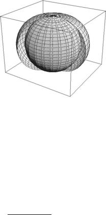
Fig. 3.4 The static limit surface ΣSL defined by
r = r+(θ ) is an ellipsoid and contains inside itself the
spherical surface
r = rH = r+( π2 ) which, as we discuss in the main text, is the event horizon ΣH . The static limit surface is tangential to the horizon at the North and South poles of the hole. The region contained between ΣSL and ΣH is named the ergosphere
form (3.3.7). When the discriminant of that quadratic form vanishes, the two-roots coincide and we have:
Ωmax = Ωmin = ΩH |
(3.4.1) |
Inspecting (3.3.7) we see that its discriminant is given by the expression: |
|
= gt2φ − gtt gφφ = r2 + α2 − 2mr + q2 |
(3.4.2) |
which is indeed the building block function Δ(r) introduced in (3.2.2). The reason for the choice of its name becomes now apparent.
We claim that the bigger root of the quadratic equation Δ(r) = 0 is the eventhorizon of the black-hole. Let us first spell out the two roots and then motivate our
statement. We have |
|
= 0 → r = r± = m ± m2 − q2 + α2 |
(3.4.3) |
Let us now argue in the following way. Given the two Killing vectors (3.3.1) let us define the family of Killing fields:
χ (Ω) |
= k + Ω ˜ |
(3.4.4) |
k |
which, as we know from (3.3.6), correspond to the 4-velocities of test-bodies having angular velocities Ω with respect to the fixed stars. For each χ (Ω) let us consider the light-like radial curves that admit χ (Ω) as the tangent vector field. Explicitly we set:
dt = dp; dφ = Ω dp; dθ |
(3.4.5) |
and we obtain the equation:
0 = gtt dp2 + 2Ωgtφ dp2 + Ω2gφφ dp2 + grr dr2 |
(3.4.6) |
so that for each Ω we have an effective 2-dimensional metric:
ds2 = gpp(r, Ω) dp2 + grr dr2 |
(3.4.7) |