


4.5 The Cosmic Background Radiation |
91 |
Fig. 4.17 The behavior of the scale factor in a matter filled universe for the three cases of positive, negative and null spatial curvature
into a state of infinite energy density. The Big Bang is followed, in the closed universe, by a Big Crunch.
These are the implications, visually summarized in Fig. 4.17 and accurately derived in the next chapter, of the Cosmological Principle, namely of the assumption that the Universe is isotropic and homogeneous. Is it really such?
4.5 The Cosmic Background Radiation
The final answer to the question posed at the end of the previous subsection came in 1965 thanks to Arno Allan Penzias and Robert Woodrow Wilson who, for their discovery of that year were awarded the Nobel Prize in 1978.
Penzias was born in a Jewish family in Munich in 1933, the very same year when Hitler got to power. Wilson was born three years later in that Texas which at the end of World-War Two boasted the victory on Germany, as a contemporary newspaper ironically wrote one of those days: Texas has defeated the Third Reich.
In 1939 Arno Penzias was among the 10.000 Jewish children who were evacuated from Germany and transported to England with the naval operation later known as Kindertransport. He was luckier than the majority of his fellow travelers who lost their parents and relatives in the Nazi lagers of the Holocaust. Arno’s father and mother succeeded to flee to the United States just six months later than the evacuation of their son who could reach them in New York. There he lived, studied and in 1962 he got his Ph.D. at Columbia University.
Penzias and Wilson, who had obtained his Ph.D. from the California Institute of Technology at Pasadena, met a short time later at the Laboratories of the Bell Telephone Company in New Jersey. Both young researchers had been hired by Bell and in the little village of Holmdel, near the Company Headquarters at Crawford Hill, they worked at the construction of a new large radio antenna. The Horn Antenna

92 |
4 Cosmology: A Historical Outline from Kant to WMAP and PLANCK |
Fig. 4.18 The two discoverers of the Cosmic Background Radiation, Penzias and Wilson with their instrument, the Horn Antenna
they had designed was conceived for experiments in radioastronomy and telecommunications between the Earth and the artificial satellites (see Fig. 4.18). However there was a problem.
The sophisticated apparatus displayed an excess of antenna temperature of 3.5 Kelvin degrees that the two brilliant engineers could not explain. From Crawford Hill they phoned Princeton University and discussed their problem with Dicke, Wilkinson and Roll who were constructing another similar radio antenna. Immediately after that conversation Dicke exclaimed to his collaborators: Guys, they got it! They made the scoop! Which was the scoop alluded to by that distinguished professor who, during World War Two, at the Radiation Laboratory of the MIT, had
4.5 The Cosmic Background Radiation |
93 |
Fig. 4.19 Alexander Friedman (1888–1925) and his student Georgij Gamow (1904–1968)
created the Dicke radiometer, a sophisticated detector of electromagnetic waves? The scoop was the discovery of the Cosmic Background Radiation. With great intuition Dicke had immediately guessed the origin of that 3.5 K excess. No terrestrial phenomenon and no instrumental error could explain it. Behind that ultra-cold remnant lurked a cosmic phenomenon that had been predicted, few decades before by another brilliant fugitive.
Georgij Antonovich Gamow (see Fig. 4.19) was born from Russian parents in 1904 in the imperial town of Odessa, refunded in 1794 by Catherine the Great on the ruins of the Turkish Town of Khadjibey, just captured by the Russians from the Ottomans. At the beginning Gamow studied in his natal town at the University of Novorossya, but in 1922 he went to Saint Petersburg, transformed into Leningrad after the October Revolution. Here he became student of Alexander Friedman.
This latter, a brilliant Russian Mathematician and Physicist, spent the whole of its life in Leningrad and prematurely died at the age of thirty-seven in 1925. His name corresponds to the F in the denomination of the standard cosmological metric. In a 1924 article, published in German on the Zeitshrift für Physik and bearing the title
Uber die Möglichkeit einer Welt mit konstanter negativer Krümmung,1 Friedman, independently from Lemaitre, presented the cosmological solutions, isotropic and homogeneous, of the Einstein equations for the three cases of positive, negative and null curvature (κ = ±1, 0) [5]. Robertson and Walker reobtained the same solutions ten years later. It is also interesting to stress that the mathematical solution of 1924
1On the possibility of a world with negative spatial curvature.

94 |
4 Cosmology: A Historical Outline from Kant to WMAP and PLANCK |
had no motivation in experimental data since Hubble’s law was discovered only five years later when Friedman was already dead.
In Leningrad, Gamow, who lost his thesis advisor before the end of his Ph.D., obtained in 1929, established a close friendship relation with another student who was to become one of the greatest physicists of the XXth century: Lev Davidovich Landau. Nobel laureate in 1962 for its theory of superfluidity, Landau was the greatest master of Soviet Physics and the endless series of volumes of his course on theoretical physics, written with his younger collaborator Lifshitz has been the educational basis of thousand of physicists around the world.
As for intellectual phantasy and scientific successes, Gamow was not that much inferior to his friend Landau. Differently from the latter who, except for two short trips to Copenhagen and Zürich, never left the Soviet Union, and suffered also one year in jail at the time of Stalin Purges, Gamow, who had worked both in Copenhagen and Göttingen tried to emigrate as early as 1932. With his wife he tried an escape on a small boat once on the Black Sea towards Turkey, a second time from Murmansk to Norway. Both times they failed because of very bad weather conditions, but in 1933 the Gamows succeeded in their intent having obtained from Soviet authorities the permission to participate to one of the famous Solvay Conferences in Brussels. There they deserted the Soviet Union and became political refugees. In 1934 from Belgium they went to the United States where, becoming Americans, they spent the rest of their life.
Gamow contributed fundamental results in nuclear physics explaining the β- decay of heavy nuclei and was the inventor of the drop model of the nucleus.
In a paper [6], based on previous results of Alpher [7] and published in 1948 on the Physical Review, Gamow advocated that the Universe should be filled with an electromagnetic Black Body radiation produced by all the atomic and subatomic transitions occurred after the Big Bang. For a certain period during the cosmic expansion this primeval radiation was in thermal equilibrium with ionized matter and the rest of the energy content of the Universe. However, as the expansion went on, the primeval radiation fell out of equilibrium with matter that had recombined into atoms and had become too rarefied in order to interact with radiation. Since that moment, known as the decoupling time, the cosmic radiation became, according to Gamow, a fossil which pervades the entire space-time but essentially does not interact with anything. Furthermore because of the cosmological red-shift, due to the universe expansion, which stretches all the wave-lengths,2 the effective black-body temperature of the fossil radiation has cooled down to incredibly low values, close to the absolute zero. Indeed knowing the age of the universe through Hubble’s law, Alpher and Gamow evaluated the red-shift factor and predicted that the Cosmic Microwave Background Radiation should have a black-body temperature of the order of few Kelvins. They advanced the prediction of 5 K.
In an almost accidental way, Penzias and Wilson had discovered the primeval radiation predicted by Alpher and Gamow. Its temperature was not exactly 5 K but very close to such number. In the first estimate of the discoverers 3.5 K, in
2The cosmological redshift will be explained in mathematical terms in later sections, at the end of this historical introduction.

4.5 The Cosmic Background Radiation |
95 |
subsequent more precise measurements 2.75 K. Dicke, Wilkinson and Roll were constructing a Dicke radiometer in order to detect this cosmic background but they were not fast enough. Penzias and Wilson had made the scoop and for that scoop they were awarded the 1978 Nobel Prize in Physics.
The 1965 detection of the CMB (Cosmic Microwave Background) not only confirmed Gamow hypothesis and gave the first direct evidence of the Big Bang but also provided an image of the primeval Universe.
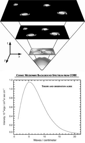
Thirteen billion of years old, the CMB is the light emitted by the Last Scattering Surface (LSS). By this name we denote the space occupied by the entire energy content of the Universe at the time of decoupling. Hence the spatial distribution of the CMB at the present time is a quite faithful image of the spatial distribution of light sources at that very remote age. As it was immediately evident at that time and as we could later verify with incredibly high precision, the CMB presents an absolutely perfect black-body spectrum. The distribution of the energy amplitude emitted at frequency ν, for unit of surface, unit of solid angle and unit of time, follows the Planck curve (see Fig. 4.20). The experimental data for the CMB are reproduced with incredibly high accuracy by the Planck curve corresponding to temperature T = 2.725 K and this happens in the same way independently from the direction in which our spectrometer points.
Recalling that what we see through the CMB is a uniformly redshifted image of the LSS, namely of the primeval Universe we can conclude that this latter was absolutely homogeneous and isotropic to a very high accuracy.
Therefore the detection of the CMB has been the experimental confirmation of the Cosmological Principle. The Universe where we live has evolved from an isotropic and homogeneous state and therefore is accurately described by a FLRW metric. Assuming this latter, the Einstein equations imply without any possible escape the expansion of the Universe, presently visible through the Hubble law. That this expansion occurred through the last thirteen billion of years is also confirmed by the gigantic redshift of the CMB. Starting from a temperature of about 3000 K that was that of the Universe at the decoupling time, corresponding to about 400.000 years after the Big Bang, in the following 13 billions of years the radiation cooled down to the present T = 2.725 K.
A trivial calculation provides a shaking evidence of this truth. As we shall prove
ae |
|
where νe |
is the fre- |
later on, the cosmological redshift goes as follows ν0 = a0 |
νe |
quency of a photon at the time of emission in the remote past while ν0 is the frequency of the same photon detected at the present time. Similarly a0 and ae denote the values of the scale factor at the two considered instants of time. From this consideration it follows that the temperature of the cosmic black-body radiation follows the same law and we have:
|
|
|
Te |
a0 |
|
||
|
|
|
|
|
= ae |
(4.5.1) |
|
|
|
T0 |
|||||
From this we obtain the estimate: |
|
|
|
|
|
|
|
|
a0 |
3000 |
103 |
|
|||
|
|
|
|
(4.5.2) |
|||
|
ae |
2.725 |
|||||
96 |
4 Cosmology: A Historical Outline from Kant to WMAP and PLANCK |
Fig. 4.20 The perfect
Black-Body spectrum of the
Cosmic Microwave
Background Radiation
On the other hand the ratio between the two considered times is:
t0 |
|
13 × 109 |
|
3 |
|
104 |
|
104.5 |
(4.5.3) |
|
te |
|
4 × 10⁵ |
× |
|
||||||
|
|
|
|
|||||||
According to Friedman equations, the asymptotic behavior of the scale factor in a flat matter dominate universe is a t2/3. Now it is remarkable that:
104.5 32 103 |
(4.5.4) |
In other words the observed redshift of the CMB over the last 12.5 billions of years from the decoupling is consistent with the expansion of the universe predicted by Friedman equations in the case of a flat, matter dominated Universe.