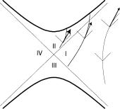
Fig. 2.9 The light-cone orientations in Kruskal space-time and the difference between physical geodesics in regions I and II

its inclination α with respect to the X axis is in the following range 3π/4 ≥ α ≥ π/4. This applies to the whole plane, yet it implies a fundamental difference in the destiny of physical particles that start their journey in region I (or IV) of the Kruskal plane, with respect to the destiny of those ones that happen to be in region II at some point of their life. As it is visually evident from Fig. 2.9, in region I we can have curves (and in particular geodesics) whose tangent vector is time-like and future oriented at any of their points which nonetheless avoid the singular locus and escape to infinity. In the same region there are also future oriented time-like curves which cross the horizon X = ±T and end up on the singular locus, yet these are not the only ones, as already remarked. On the contrary all curves that at some point happen to be inside region II can no longer escape to infinity since, in order to be able to do so, their tangent vector should be space-like, at least at some of their points. Hence the horizon can be crossed from region I to region II, never in the opposite direction. This leads to the existence of a Black-Hole, namely a space-time region, (II in our case) where gravity is so strong that not even light can escape from it. No signal from region II can reach a distant observer located in region I who therefore perceives only the presence of the gravitational field of the black hole swapping infalling matter.

To encode the ideas intuitively described in this section into a rigorous mathematical framework we proceed next to implement our already announced programme. This is the critical review of the concepts of Future, Past and Causality within General Relativity, namely when we assume that all physical events are points p in a pseudo-Riemannian manifold (M , g) with a Lorentzian signature.

2.3 Basic Concepts about Future, Past and Causality

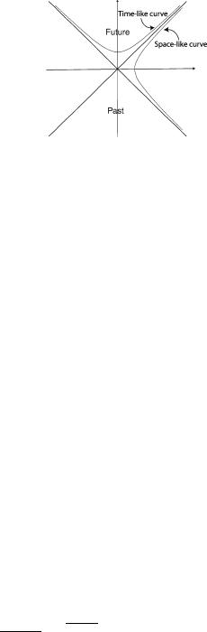
Our discussion starts by reviewing the basic properties of the light-cone (see Fig. 2.10). In Special Relativity, where space-time is Minkowski-space, namely a pseudo-Riemannian manifold which is also affine, the light cone has a global meaning, while in General Relativity light-cones can be defined only locally, namely at each point p M . In any case the Lorentzian signature of the metric implies thatp M , the tangent space Tp M is isomorphic to Minkowski space and it admits the same decomposition in time-like, null-like and space-like sub-manifolds. Hence

Fig. 2.10 The structure of the light-cone

the analysis of the light-cone properties has a general meaning also in General Relativity, although such analysis needs to be repeated at each point. All the complexities inherent with the notion of global causality arise from the need of gluing together the locally defined light-cones. We will develop appropriate conceptual tools to manage such a gluing after our review of the local light-cone properties.

2.3.1 The Light-Cone

When a metric has a Lorentzian signature, vectors t can be of three-types:

1.Time-like, if (t, t) < 0 in mostly plus convention for gμν .

2.Space-like, if (t, t) > 0 in mostly plus convention for gμν .

3.Null-like, if (t, t) = 0 both in mostly plus and mostly minus convention for gμν .

At any point p M the light-cone Cp is composed by the set of vectors t Tp M which are either time-like or null-like. In order to study the properties of the lightcones it is convenient to review a few elementary but basic properties of vectors in Minkowski space.

Theorem 2.3.1 All vectors orthogonal to a time-like vector are space-like.

Proof Using a mostly plus signature, we can go to a diagonal basis such that:

Lemma 2.3.1 The sum of two future-directed time-like vectors is a future-directed time-like vector.

Proof Let t and T be the two vectors under considerations. By hypothesis we have

which proves that t + T is time-like. Moreover t0 + T 0 > 0 and so the sum vector is also future-directed as advocated by the lemma.

On the other hand with obvious changes in the proof of Theorem 2.3.1 the following lemma is established

Lemma 2.3.2 All vectors X, orthogonal to a light-like vector L are either light-like or space-like.

Let us now consider in the manifold (M , g) surfaces Σ defined by the vanishing of some smooth function of the local coordinates:

By definition the normal vector to the surface Σ is the gradient of the function f :