

5.3 Homogeneity Without Isotropy: What Might Happen |
141 |
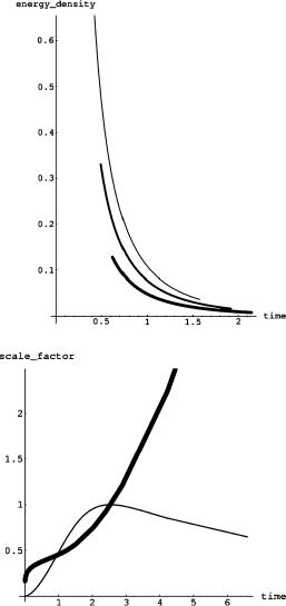
Fig. 5.10 The evolution of the energy density of the scalar field as function of the cosmic time, for various values of κ. The bigger κ, the thinner the corresponding line. Here κ = 0.5 is the thickest line. The other two correspond to κ = 0.7 and
κ = 1, respectively
Fig. 5.11 The evolution of the two scale factors as function of the cosmic time τ in the dilaton gravity solution. The thicker line is Λ while the thinner one is . The chosen value of the parameter kappa is κ = 0.7
5.3.5 Three-Space Geometry of This Toy Model
In order to better appreciate the structure of the cosmological solutions we have been considering in the previous subsection it is convenient to study the geometry of the constant time sections and the shape of its geodesics. At every instant of time we have the 3D-metric:
ds32D = Λ dx2 + dy2 + |
dz + |
ω |
(x dy − y dx) |
2 |
|
(5.3.67) |
|||||
|
|||||
4 |
142 |
5 Cosmology and General Relativity |
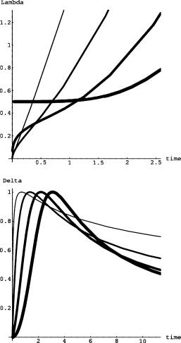
Fig. 5.12 The evolution of the Λ scale factor as function of the cosmic time τ in the dilaton gravity solution and for different values of kappa. The thickest line corresponds to κ = 0. The bigger κ, the thinner the line as in the other plots. Here we have
κ = 0, 1, 2, 4. For all κ = 0, Λ begins at zero
Fig. 5.13 The evolution of the scale factor as function of the cosmic time τ in the dilaton gravity solution and for different values of kappa. The bigger κ, the thinner the line. Here we have
κ = 0, 1, 2, 4. has always the same behavior and increasing κ corresponds only to an anticipation of the peak
which admits the Killing vectors (5.3.27) as generators of isometries. As we explained several times, the scalar product of Killing vectors with the tangent vector
to a geodesic is constant along the geodesic. Hence if λ is the affine parameter along |
|||||||||||||||||||||||||||
a geodesic and |
−→ |
= { |
x |
[ ] |
, y |
[ ] |
[ |
λ |
]} |
is the tangent vector to the same, then we |
|||||||||||||||||
|
|
|
t |
|
|
|
λ |
|
λ , z |
|
|
|
|||||||||||||||
have the following four constants of motion: |
|
|
+ |
|
|
|
|
|
|||||||||||||||||||
A1 (−→1 |
−→ |
|
|
|
− |
(ωy(λ)x (λ)) |
+ |
ωx(λ)y |
(λ) |
4z (λ)) |
|
|
|||||||||||||||
≡ |
k |
, t ) |
= |
|
Δ( |
|
|
|
|
|
|
|
|||||||||||||||
|
|
|
|
|
|
|
|
|
|
|
|
4 |
|
|
|
|
|
|
|
|
|
|
|
||||
|
|
|
|
|
|
|
|
|
|
|
|
|
|
|
|
|
|
|
|
|
|
|
|
|
|
||
A2 ≡ (−→O |
−→ |
= |
16 |
|
|
+ |
|
|
|
|
|
|
|
|
|
|
+ |
|
|
|
|||||||
|
k |
, t ) |
|
1 |
|
|
16Λ |
|
|
Δω2x(λ)2 |
y(λ)x |
(λ) |
|
|
Δω2y(λ)3x |
(λ) |
|
||||||||||
|
|
|
|
|
|
|
|
|
|
|
|||||||||||||||||
|
|
|
|
|
− Δωy(λ)2 ωx(λ)y (λ) + 4z (λ) |
|
|
|
|
|
|||||||||||||||||
|
|
|
|
|
− x(λ) 16Λ + Δω2x(λ)2 y (λ) + 4Δωx(λ)z (λ) |
(5.3.68) |
|||||||||||||||||||||

5.3 Homogeneity Without Isotropy: What Might Happen |
|
|
|
|
|
|
|
143 |
||||||||||||||||||||
A3 |
≡ |
(−→2 |
|
−→ |
|
= |
(8Λ |
+ |
Δω2y(λ)2)x (λ) |
− |
Δωy(λ)(ωx(λ)y (λ) |
+ |
4z (λ)) |
|
||||||||||||||
|
|
k |
, |
t |
) |
|
|
|
8Λy (λ) |
+ |
Δω2x(λ)2y (λ) |
+ |
|
− |
(ωy(λ)x (λ)) |
+ |
4z (λ)) |
|||||||||||
A4 |
≡ |
(−→3 |
|
−→ |
|
= |
Δωx(λ)( |
|||||||||||||||||||||
|
|
k |
, |
t |
) |
|
|
|
|
|
|
|
|
|
|
|
|
|
|
|
|
|
|
|
|
|
|
|
Then the geodesics are characterized by the equations: |
|
|
|
|
|
|
|
|
|
|
||||||||||||||||||
|
|
|
A |
2 |
= |
|
−4A4x(λ) + 4A3y(λ) + ωA1(x(λ)2 + y(λ)2) |
|
|
|
|
|
(5.3.69) |
|||||||||||||||
|
|
|
|
|
|
|
||||||||||||||||||||||
|
|
|
|
|
|
|
|
|
|
|
4 |
|
|
|
|
|
|
|
|
|
|
|
|
|
|
|||
and |
|
|
|
|
|
|
|
|
|
|
|
|
|
|
|
|
|
|
|
|
|
|
|
|
|
|
|
|
|
|
|
z (λ) |
= |
8ΔωA2 + A1(8Λ − Δω2x(λ)2 − Δω2y(λ)2) |
|
|
|
|
(5.3.70) |
||||||||||||||||||
|
|
|
|
|
|
|
||||||||||||||||||||||
|
|
|
|
|
|
|
|
|
|
|
8ΔΛ |
|
|
|
|
|
|
|
|
|
|
|
|
|
||||
We also have:
x (λ) = 2A3 + ωA1y(λ)
2Λ
y (λ) = 2A4 − ωA1x(λ)
2Λ
We conclude that the projection of all geodesics on the centers at:
|
0 |
0 |
|
|
= |
ωA1 |
ωA1 |
|
|
||
(x |
, y |
) |
|
|
2A4 |
, |
−2A3 |
|
|
||
|
|
|
|
|
|
||||||
and radii: |
|
|
|
|
|
|
|
|
|
|
|
|
|
|
|
|
|||||||
R |
= |
2/ |
ωA1A2 + A32 + A42 |
||||||||
|
|
|
|
|
|
ω2A12 |
|
|
|||
(5.3.71)
xy plane are circles with
(5.3.72)
(5.3.73)
and in terms of the new geometrically identified constants (5.3.70) becomes:
z (λ) |
= |
A1(8Λ + 2Δω2(R2 − x02 − y02) − Δω2x(λ)2 − Δω2y(λ)2) |
(5.3.74) |
|
|||
|
8ΔΛ |
||
If we use a polar coordinate system in the xy-plane, namely if we write:
x0 = ρ cos[θ ]; |
y0 = ρ sin[θ ] |
(5.3.75) |
x = ρ cos[θ ] + R cos φ(λ) ; |
x = ρ sin[θ ] + R sin φ(λ) |
|
where ρ and θ are constant parameters, we obtain that the derivative of the angle φ with respect to the affine parameter λ is just:
dφ |
= − |
ωA1 |
(5.3.76) |
dλ |
2Λ |
144 |
5 Cosmology and General Relativity |
Fig. 5.14 In the first picture we see two geodesics in three space, while in the second we see their projection onto the plane xy
This means that φ itself, being linearly related to λ, is an affine parameter. On the other hand, the equation for the coordinate z, (5.3.70), becomes:
dz |
= |
−(8Λ + Δ(R2 − 3ρ2)ω2 − 2RΔρω2 cos(θ − ϕ(λ))) |
(5.3.77) |
|
dφ |
4Δω |
|||
|
which is immediately integrated and yields:
z φ |
(θ − ϕ)(8Λ + Δ(R2 − 3ρ2)ω2) − 2RΔρω2 sin(θ − ϕ) |
(5.3.78) |
|
4Δω |
|||
[ ] = |
|
Hence the possible geodesic curves in the three-dimensional sections of the cosmological solutions we have been discussing are described by (5.3.78) plus the second of (5.3.75). The family of such geodesics is parameterized by {R, θ, ρ}, namely by the position of the center in the xy plane and by the radius. The shape of such geodesics is that of spirals (see Fig. 5.14).
A more illuminating visualization of this three-dimensional geometry is provided by the picture of a congruence of geodesics. Given a point in this 3D space, we can

5.3 Homogeneity Without Isotropy: What Might Happen |
145 |
Fig. 5.15 In this picture we present a congruence of geodesics for the space with Λ = = ω = 1. All the curves start from the same point and are distinguished by the value of the radius R in their circular projection onto the xy plane
consider all the geodesics that begin at that point and that have a radius R falling in some interval:
RA < R < RB |
(5.3.79) |
Following each of them for some amount of parametric time λ we generate a two dimensional surface. An example is given in Fig. 5.15.
The evolution of the Universe can now be illustrated by its effect on a congruence of geodesics. Chosen a congruence like in Fig. 5.15, the shape of the surface generated by such a congruence depends on the value of the scale parameters Λ and . We can follow the evolution of the congruence while the Universe expands obtaining a movie.
Having illustrated the shape and the properties of the geodesics for the three dimensional sections of space-time we can now address the question of geodesics for the full space-time. To this effect we calculate first the three dimensional line element along the geodesics and we obtain the following result
d 2(t, λ)
dλ2
|
|
|
|
|
|
|
|
|
|
|
|
ω |
|
|
|
|
2 |
|
≡ |
|
˙ |
|
|
+ ˙ |
|
+ |
˙ + |
|
˙ − |
˙ |
|
|
|||||
|
Λ(t) x |
2(λ) |
|
|
y |
2 |
(λ) |
Δ(t) z(λ) |
|
|
|
|
x(λ)y(λ) |
y(λ)x(λ) |
|
|
||
|
|
|
|
|
4 |
|
|
|||||||||||
|
(16R2Λ(t)ω2 |
+ |
(−8Λ(t)+3Δ(t)ρ2ω2+3RΔ(t)ρω2 cos(θ −ϕ(λ)))2 )A 2 |
|
||||||||||||||
= |
|
|
|
|
|
|
|
|
Δ(t) |
|
|
1 |
|
|
||||
|
|
|
|
|
|
|
|
|
64Λ(t)2 |
|
|
|
|
|
|
|
|
|
|
|
|
|
dφ |
|
2 |
|
|
|
|
|
|
|
|
|
|
||
≡ F 2(t, φ) |
|
|
|
|
|
|
|
|
|
|
(5.3.80) |
|||||||
dλ |
|
|
|
|
|
|
|
|
||||||||||
In the last step of (5.3.80) we have introduced the notation:
F 2 |
|
(16R2 |
Λ(t)ω2 |
+ |
(−8Λ(t)+3Δ(t)ρ2ω2+3RΔ(t)ρω2 cos(θ −ϕ(λ)))2 ) |
|
||
(t, φ) = |
|
|
|
Δ(t) |
(5.3.81) |
|||
|
|
|
16ω2 |
|
|
|||
and we have used the relation (5.3.76).