4.3.4 The Big Bang

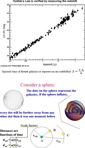
How was Hubble’s Law derived and how can it be verified? The answer is by means of the redshift of atomic spectral lines.

In order to clarify this point it is convenient to consider its analogy with the familiar Doppler effect in acoustical waves. We all made experience of what happens when an ambulance goes by, horning his siren. When the vehicle approaches the tune of its siren is high pitched while, when it runs away from us, the siren tune falls off and off. Moreover the faster the vehicle runs away, the lower falls the tune. The same happens for light waves, namely for photons.

The faster a luminous source recedes from an observer the redder it appears to him. Hence by performing the spectral analysis of the light which comes to us from distant galaxies we can recognize the structure of spectral lines for all atomic transitions but we also find that they are all shifted towards low frequencies and that they are the more shifted the larger is the distance of the observed galaxy. Defining redshift the percentual change of spectral lines and plotting it against the distance one obtains a line whose slope is Hubble’s constant H0.

Hence the redshift factor is defined:

where λ is the wave-length of a spectral line observed in a distant galaxy while λ0 is the wave-length of the corresponding spectral line observed in laboratory experiments on the Earth (see Fig. 4.11).

What is the interpretation of Hubble’s Law?

At first sight one might think that it denotes our privileged position in the Universe. If all cosmic objects radially recede from us, it follows that we are at the center of the Universe which, once upon a time, was all concentrated in the place where we are now. Furthermore a linear relation between the recession velocity and the distance suggests the scenario of a gigantic primeval explosion. At the time when a bomb explodes all of his fragments are expelled in all directions with different velocities. After some time the faster fragments have run the further and for this reason they are more distant.

This interpretation which corresponds to an anthropic principle is what suggested the naming BIG BANG, yet it is somehow naive and conflicts with the homogeneity and isotropy of the Universe. As a consequence of this homogeneity and isotropy we should rather suppose that what we see is exactly the same picture seen by any other observer in any other galaxy. How can we then interpret Hubble’s Law?

The intuitive model is the following one.

The galaxies are like balls arranged on a elastic sheet (the three-dimensional space) and with respect to that sheet they do not move. Yet it is that sheet that is uniformly stretched in all directions and as a consequence of this stretching every ball recedes from every other one. This way of thinking leads us to the concept of time dependent scale-factor (see Fig. 4.12). Imagine that our three-dimensional

Fig. 4.11 The redshift of distant galaxies

Fig. 4.12 The expansion of three-dimensional space

space is something like the surface of a two-sphere and that the galaxies are arranged and soldered at fixed locations on that spherical surface. Let us now imagine that some demon inflates the sphere, namely that he enlarges its radius while times goes on. All distances between each of the galaxies with all the others have fixed ratios but they are all proportional to the radius of the sphere which grows in time and so they also uniformly grow. It is like if the unit of measure increased constantly and were a function of time. We denote this time dependent unit of measure the scale factor and we denote it as a(t).

Velocity is the derivative of the distance with respect to time. A simple calculation shows that we can deduce Hubble’s Law from the above reasoning and identify Hubble’s constant with the logarithmic derivative of the scale factor at the present