5.10 The Anisotropies of the Cosmic Microwave Background

5.10 The Anisotropies of the Cosmic Microwave Background

Let us consider a spatially flat Universe described, in the conformal frame, by the following metric:

Small perturbations of the above metric can be organized according to their spin (s = 0, 1, 2). Dominant contributions to physically observable phenomena are the lowest spin ones, namely the scalar fluctuations. As we have seen in Sect. 5.9, modulo gauge-transformations corresponding to diffeomorphisms, such scalar perturbations can be encoded into a potential function Φ(η, x) that deforms the homogeneous isotropic metric (5.10.1) in the following way:

Perturbation means that Φ(η, x) ' 1. The relativistic potential Φ plays a role very similar to that of the Newtonian potential and it describes local variations of the average gravitational field that can be somewhat stronger here and somewhat weaker there. In Sect. 5.9 we discussed the relation between Φ and the single quantized scalar degree of freedom of the Einstein-Klein-Gordon system. It is an incredibly interesting fact that such inhomogeneities of the average gravitational field can be directly observed as fluctuations in the temperature of the cosmic background radiation. Not only that: the relation between temperature fluctuations and fluctuations of the gravitational field is preserved during cosmic evolution so that, by observing present day inhomogeneities of the CMB, we directly measure the inhomogeneities of the gravitational field at the time of recombination or last scattering, namely when electromagnetic radiation fell off thermal equilibrium with respect to baryon matter. According to the thermal history of the Universe, this happened about 400 thousand years after the Big Bang, namely about 14 billion years ago. This crucial link between Φ and the temperature fluctuations is named the Sachs-Wolfe effect whose derivation is the issue addressed in the following subsection.

5.10.1 The Sachs-Wolfe Effect

Let us define the distribution function f (xi , pi , η) which informs us about the number of photons dN at time η, which have three-momentum pi at place xi :

When we deal with a black-body radiation, like the cosmic background one, the distribution function is Planckian and we have:

where T (x, n) is the temperature, which can depend both on the place x and on the direction n in which we observe the thermal spectrum, and ω is the energy of the considered photon. Calling uα the four-velocity of the observer and pα the fourmomentum of the photon the energy measured by the observer is given by:

Naming p = pi the spatial part of the momentum and calling:

we can easily calculate ω in the reference frame where the observer is at rest, namely uα = {√g00, 0, 0, 0}. Since the photon is a massless particle we have pα pβ gαβ = 0 which in the metric (5.10.2) implies

Φ'1

the last identity corresponding to the first order contribution in the perturbation Φ. For any metric, the distribution function must obey the Boltzmann transport

equation:

which, as specified by the last equality in (5.10.9), is the statement that the total time derivative of f should vanish so that the total number of photons in the Universe is conserved.

Equation (5.10.9) can be simplified using the explicit form of the metric and the equation for null geodesics that are those traveled by the photons. Naming λ an affine parameter along the geodesics, the four-momentum vector of the photon can be identified as:

and, relying on the explicit form of the Christoffel symbols, the geodesic equation takes the following form:

Then (5.10.9) is rewritten as:

In the metric (5.10.2), from the null-like condition pα pβ gαβ = 0 we derive the result:

Developing (5.10.15) to first order in the small perturbation Φ we obtain the approximate transport equation:

Let us apply the above transport equation to the Planckian distribution function (5.10.4). It reads as follows:

The quantity Q can be developed in power series of the perturbations. As for the photon energy ω we have already derived such a development in (5.10.8) that can be restated as follows:

where the 0th order term ω0 depends only on time being homogeneous and isotropic, while the perturbation δω(η, x) varies from place to place. We can introduce a similar development for the CMB temperature:

Combining (5.10.20) and (5.10.21) we obtain:

Inserting the above development of Q into the transport equation (5.10.18), at 0th order we obtain:

∂ −1 =

a(η)T0(η) 0 (5.10.23)

∂η

while at first order in the perturbations we get:

Equation (5.10.23) implies that the average temperature of the cosmic background radiation is a monotonic function of the cosmic time and decreases inversely to the scale factor while the Universe expands. In other words the temperature T0 is a very precise cosmological clock. On the other hand (5.10.24) for the perturbation has a very simple and most profound interpretation. It suffices to note that the operator

is just a total time derivative. Hence if the relativistic potential Φ(x) depends only on space and not on time, then the combination

is constant not only in time but also in space, as a consequence of (5.10.24). There-

fore, measuring the inhomogeneities of the CMB temperature δT at our time is the

T0

same thing as measuring the inhomogeneities of the gravitational potential Φ at the last scattering time 14 billions of years ago. The spectrum of such perturbations is predicted by the theory of inflation which therefore becomes, to a certain extent, experimentally verifiable.

5.10.2 The Two-Point Temperature Correlation Function

What is actually observed by CMB experiments is the spatial distribution of the

temperature fluctuations, namely δT (n), having denoted by n a unit vector on the

T0

three-sphere, just as we did in the previous section. Using these data, that are visualized in sky-maps like that of Fig. 4.24, one can construct the correlation function:

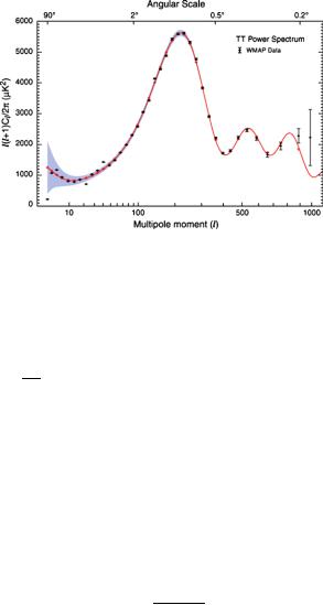
Fig. 5.31 Dependence of the CMB anisotropy multipole moments on , as measured by the WMAP satellite

where the bracket ! denotes averaging over all directions of the sky n1 and n2 satisfying:

Next the correlation function is expanded in multipoles by setting:

∞

C(θ ) = 1 (2 + 1)C P (cos θ ) (5.10.29) 4π =2

and the experimental data are encoded in the angular momentum dependence of the multipole moment C , producing a graph such as that displayed in Fig. 5.31 (see [10–14]). Note that the multipole expansion excludes the first two moments, the monopole = 0 and the dipole = 1, which are sensitive to the position of the Sun in the Galaxy and to its motion around the Galaxy center. All the other moments automatically exclude these effects and provide therefore a clean information on primeval perturbations. The existence of the Sachs Wolfe effect allows to write down an analytic formula which predicts the multipole coefficients in terms of power spectrum we discussed in the previous section. Explicitly one finds:

The ingredients entering the above formula are:

1.By ηr we denote the conformal time of recombination, after which the background radiation fell off equilibrium with matter.

2.By η0r we denote the present conformal time at which we observe CMB.

3.By σκ (η) we denote the Fourier component of the scalar potential Φ defined in (5.9.70), from which the power spectrum is calculated according to (5.9.73).

4.By j (r) we denote the spherical Bessel functions.

5.The two functions δκ (ηr ) and δκ (ηr ) encode a description of the CMB temperature fluctuations at the time of recombination.