


4.6 The New Scenario of the Inflationary Universe |
97 |
4.6 The New Scenario of the Inflationary Universe
The great success of the Standard Cosmological Model, based on the hypothesis of the hot Big Bang and the principles of homogeneity and isotropy, which are mathematically rephrased by assuming the FLRW metric (4.4.1), should not induce the reader to think that everything has been understood and solved. In Physics the absolute agreement of a theoretical model with experimental data is often the source of a conceptual problem, rather than being its solution.
At first sight, such a statement might seem paradoxical, yet a short discussion can clarify its profound meaning. If reality agrees perfectly and not only approximately with some modeling of its behavior, that means that the hypothesis underlying our model do not correspond to some accidental circumstances, rather to some fundamental law, and the problem is that of explaining such a law in terms of more profound reasons and principles. A historical example is that of the identity between the inertial and the gravitational mass. These latter are not approximately equal rather they are equal with extraordinary precision. This means that a good theory of gravitation should include such an identity as a necessary and founding condition, not as an accidental fact. Starting from this consideration, as we know, Einstein discovered General Relativity.
Similarly the Standard Model of Strong, Weak and Electromagnetic Interactions has proved to be a very precise and accurate description of elementary particle physics. Yet, this model includes a large number of parameters and the problem is that of creating a more fundamental theory, within whose frame the values of the standard model parameters can be predicted equal to those experimentally measured.
In the case of Cosmology, the high accuracy of the predictions of the Big Bang Model implies the necessity of explaining in more profound terms the two hypotheses that constitute its foundation, namely homogeneity and isotropy, alias the Cosmological Principle.
Considering this issue with a clear and not biased mind, we easily convince ourselves that there is no a priori reason for the Universe to be so homogeneous and symmetric, as it proves to be in observations. On the contrary, it would be natural for it to be highly disordered and inhomogeneous. Indeed one can show that, starting from a situation that includes anisotropies and inhomogeneities, Einstein equations tend to enlarge them during time evolution. Therefore, if we confine ourselves to consider Einstein theory with a Universe content made only of conventional matter and radiation, then the extraordinary isotropy and homogeneity of the Universe at present time requires that its initial state was prepared homogeneous and isotropic with almost infinite precision, which is quite unnatural in any stochastic process.
Different is the perspective if we discover a physical mechanism that can prepare such isotropic and homogeneous state starting from a generic one.
In 2002 the Dirac Medal of Trieste ICTP,3 which, after the Nobel Prize, is probably the most prestigious honor available to theoretical physicists, was awarded to Alan Guth, Andrei Linde and Paul Steinhardt, for their fundamental contributions
3International Centre of Theoretical Physics.

98 |
4 Cosmology: A Historical Outline from Kant to WMAP and PLANCK |
Fig. 4.21 Alan Guth, Andrei Linde and Paul J. Steinhardt, the fathers of the Inflationary Universe scenario
to the creation of the Inflationary Universe paradigm (see Fig. 4.21). Alan Guth, born in the USA in 1947 is professor at the Massachussetts Institute of Technology, Paul J. Steinhardt, also born in the US, is Einstein professor of Physics at Princeton University, while Andrei Linde, born in Moscow, studied and worked there, becoming one of the most famous and distinguished cosmologists of the world. In the mid nineties of the XXth century he accepted the invitation of Stanford University to join the faculty of its Physics Department.
There are many formulations of the inflationary theory and its details crucially depend on the structure of the unified theory of all interactions that will prove to be the one chosen by Nature. For instance, within the framework of supergravity, regarded as the low-energy limit of superstring theory, there are several interesting

4.7 Great News at the End of the Second Millenium |
99 |
possibilities to implement the inflationary scenario and determine its parameters in agreement with the experimental data that are piling up. However, beyond its detailed structure, the great value of the Inflationary Universe is that it provides a very simple conceptual paradigm, up to now without any rivals, capable of explaining the isotropy, homogeneity and spatial flatness of the Universe.
Here we do not dwell too much on explanations of Inflation, which will be discussed in a detailed mathematical way in later sections. We just mention that the generic mechanism, capable of preparing homogeneous, isotropic and spatially flat boundary conditions, consists of a primeval phase of exponential expansion that should have taken place before the age of decoupling and should have also gracefully ended. On its turn, an exponential expansion takes place when gravity becomes repulsive and this happens when the energy content of the Universe is mainly provided by vacuum energy, for instance the potential energy V (ϕ) of one or more scalar fields ϕ. Hence, the inflationary universe scenario is just a generic property of any fundamental theory of particle interactions that contains scalar fields. Fundamental spin zero fields, namely scalars, have not yet been detected, but their presence is ubiquitous in all approaches to unification, they are essential in all versions of supergravity theory and they are necessary because of symmetry breaking. From this point of view we can say that Cosmology provides another indirect evidence for the existence of this type of particles whose detection is by now overdue.4
4.7The End of the Second Millennium and the Dawn of the Third Bring Great News in Cosmology
The end of the XXth century and the beginning of the XXIst brought new developments into Cosmology, almost of the same relevance as the discovery of the Hubble law in 1929. A new series of data which have become available starting from 1998 caused a substantial revolution in the subject that, by now, has entered an entirely new phase. Before 1998, theoretical Cosmology was mostly a matter of conjectures and speculations with a remote chance of verification or disproval. At the end of the next decade, in mid 2009, when the European Satellite Planck was launched from the French basis in Guyana towards the Lagrangian point L2 (see Fig. 4.25), theoretical cosmology had already evolved into a science that deals with the explanation of a series of facts established in a substantially firm way. Let us list these facts:
1.Our Universe is spatially flat.
2.Our Universe is presently in a phase of accelerating expansion.5
4July 4th 2012 it was officially announced by CERN that both ATLAS and CMS detectors had discovered a new bosonic particle that seems to be the long sought for spin zero particle implementing the Higgs symmetry breaking mechanism.
5The 2011 Nobel Prize in Physics was awarded to Saul Perlmutter of the Lawrence Berkeley National Laboratory, Brian Schmidt of the Australian National Laboratory and to Adam Reiss of the Johns Hopkins University, for their 1998 discovery of the present accelerated expansion of the Universe (see Fig. 4.22).
100 |
4 Cosmology: A Historical Outline from Kant to WMAP and PLANCK |
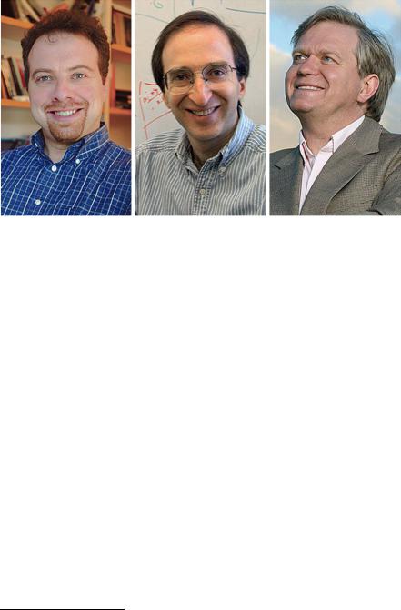
Fig. 4.22 The three recipients of the 2011 Nobel Prize in Physics that was awarded for the discovery of the present accelerated phase in the expansion of the Universe. From the right, Adam Reiss, Saul Perlmutter and Brian Schmidt
3.The energy content of our Universe is so distributed. The baryonic matter forming galaxies and providing the luminous content of the world is roughly 6 percent of the total. Dark matter, whatever it might be, amounts to about 24 percent. The remaining 70 percent, or even more, is just vacuum energy or, if you prefer, dark energy.
4.The structure of anisotropies of the CMB is in substantial agreement with the
spectrum of primeval quantum fluctuations as predicted by the inflationary scenario.6
How were these facts established?
The first very important news came around 1998–1999 with the results of two ambitious surveys of the sky, independently performed by two large international collaborations of astronomers. The two research groups, involving many observatories around the world and also the orbiting Hubble Telescope, are respectively named the Supernova Cosmology Project, which developed from an original team of Berkeley University and the High-Z Supernova Search, led by the Australia’s Mount Stromlo Observatory. Common task of the two projects was the observation of supernovae of type IA in very distant galaxies, characterized by a high redshift factor z.
Why were astronomers particularly interested in this type of exploding stars? The reason is simple and analogous to the reason that motivated Hubble to study the Cepheides in not too far galaxies. By the end of the eighties, after two decades of study of the supernova spectra, a new powerful class of standard candles had been
6The 2006 Nobel Prize in Physics was awarded to John C. Mather of the NASA Goddard Space Flight Center and to George F. Smoot, of the University of California at Berkeley for the first experimental detection of anisotropies in the Cosmic Microwave Background Radiation.

4.7 Great News at the End of the Second Millenium |
101 |
found. Indeed the spectra and the intrinsic luminosity of all known, nearby, type IA supernovae had been revealed to be equal. A fascinating theoretical explanation of these standard candles was also guessed. It was conjectured that type IA supernovae explosions originate from the following phenomenon. In a binary stellar system one of the two companions reaches the end of its life transforming first into a red-giant and then into a white dwarf, sustained against gravitational collapse by the degeneracy pressure of the electron gas, as we explained in Chap. 6 of Volume 1. The other star is still alive and active. If conditions of proximity and relative mass are right, there will be a steady stream of material from the active star slowly accreting onto the white dwarf. Over the millions of years, the dwarf’s mass increases steadily until it reaches the Chandrasekhar limit explained in Chap. 6 of Volume 1. At that point a runaway thermonuclear explosion is triggered which destroys the dwarf and manifests itself in observations as a type IA supernova. The crucial point is that the Chandrasekhar mass, whose value 1.4M is determined in terms of fundamental constants of Nature, is the same for any supernova IA. This fixes the intrinsic luminosity of the event in an absolute way giving rise to an ideal standard candle which is luminous enough to be seen also in very distant galaxies. Indeed at the time of explosion and typically for a week after that, a supernova is as luminous as an entire galaxy.
Using systematically these standard candles and surveying the sky at very high redshifts z, namely at very large distances from our observation point in the Milky Way, by the end of 1998, the two collaborations groups were ready to present their Hubble plots of the redshift versus distance which, for the first time in history, showed their deviation from linearity (see Fig. 4.23). In this way, we got the first estimate of the deceleration parameter which is defined as follows:
q |
|
|
a(t¨ 0) |
|
H |
|
|
a(t˙ 0) |
(4.7.1) |
|
0 |
≡ − a(t0)H 2 |
; |
0 |
≡ a(t0) |
||||||
|
|
|
||||||||
|
|
0 |
|
|
|
|
|
|
||
and parameterizes the aforementioned deviations. To see that, it suffices to consider the Taylor expansion of the scale factor around the present time:
a(t) = a(t0) 1 + H0(t − t0) − |
2 q0H02 |
(t − t0)2 |
+ · · · |
(4.7.2) |
|
|
1 |
|
|
|
|
and recall the definition (4.3.3) of the redshift factor which can be rewritten as follows:
z = |
λ(t0) |
− 1 = |
a(t0) |
− 1 |
(4.7.3) |
λ(t) |
a(t) |
since, as we already mentioned and as we will prove later on, the ratio between the wave-length of a photon at the present time t0 and at the time of emission t is the same as the ratio of the scale factors at the same instants of time: λ(t0)/λ(t) = a(t0)/a(t). Inserting the Taylor expansion (4.7.2) into (4.7.3) and inverting the relation we find:
cz = H0 d + |
1 + |
q0 |
H02 d2 + · · · |
(4.7.4) |
2 |
102 |
4 Cosmology: A Historical Outline from Kant to WMAP and PLANCK |
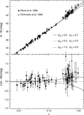
Fig. 4.23 Using type IA supernovae as standard candles and systematically detecting them in very remote galaxies has provided the means to determine the deviation of the Hubble law from linearity at high redshifts, in other words to estimate the acceleration of the Universe expansion which has proved to be positive. This is consistent with the existence of dark energy, alias of a positive cosmological constant
where c is the speed of light and the distance between us and the source as been approximated as d c(t − t0). Equation (4.7.4) presents the form of the first quadratic correction to the linear Hubble law which was experimentally evaluated for the first time in history in 1998. The surprise was immense since the deceleration parameter q0 turned out to be negative, in other words it was revealed that our Universe is actually accelerating its expansion at the present time, since a(t¨ 0) > 0.
In later sections, studying Friedman equations, we will show that the acceleration parameter can be positive only if the energy content of the Universe is dominated by vacuum energy rather than by ordinary matter and radiation. The evaluation of q0 was therefore a direct evaluation of the percentage of vacuum energy filling our Universe: approximately the 70 percent, as it turned out by taking into account the other important results about the CMB anisotropies which became available in the following years.
The satellite WMAP (Wilkinson Microwave Anisotropy Probe) was launched in June 2001 from Cape Kennedy and reached the Lagrangian point L2 wherefrom, during seven years it collected and streamed to Earth very important data on the space distribution of the Cosmic Microwave Background Radiation, in particular measuring its temperature in each direction of the sky. The oscillations of the temperature with respect to its average value T = 2.725 K are of the order of
4.7 Great News at the End of the Second Millenium |
103 |
Fig. 4.24 The microwave image of the primeval sky obtained by the seven year mission WMAP, that has measured the temperature anisotropies of the Cosmic Background Radiation. With variations of the order of few milliKelvin the microwave sky displays hotter and colder spots. As shown in later sections, the temperature variations are a direct measure of the variations in the gravitational potential at the time of decoupling, 400.000 years after the Big Bang and approximately 13 billions of years ago
the milliKelvin; when such hotter and colder spots are reported on a two-sphere representing the sky one obtains an image of the same type as shown in Fig. 4.24.
Such a plot can be regarded as an image of the Last Scattering Surface at the time of decoupling of radiation. Furthermore, because of an effect named Sachs- Wolffe-effect, which we will mathematically explain in later sections, measuring
the temperature variation function δT (x) is nothing else but measuring the primeval
T
gravitational potential Φ(x) that encodes the perturbation of the metric around its homogeneous and isotropic form.
In this way the WMAP mission, which was extremely successful, provided us with a direct measure of the cosmic primeval perturbations just before the time of radiation decoupling and established a new vision of the early Universe.
From the analysis of the CMB spectrum we learnt that our Universe is spatially flat κ = 0 and we could confirm its acceleration, obtaining a more precise evaluation of the amount of vacuum energy (around 72 %).
Furthermore the multipole analysis of the correlation function:
01
C(x − y) = |
δT (x) δT (y) |
(4.7.5) |
|
T |
T |
||
confirmed the generic predictions of the Inflationary Universe scenario showing that, with high probability, the physical mechanism which explains the mysterious homogeneity and isotropy of our Universe, alias the Cosmological Principle, is indeed the one for which the 2003 Dirac Medal was awarded. In 2009 a new radio-telescope was launched by the European Space Agency, named Planck (see Fig. 4.25). It also was placed in the Lagrangian point L2 from which it started collecting data on the CMB anisotropies with still higher precision than its predecessor

104 |
4 Cosmology: A Historical Outline from Kant to WMAP and PLANCK |
Fig. 4.25 On the left a view of the WMAP spacecraft which, for seven years, has inspected the Cosmic Microwave Background Radiation from the second Lagrangian point L2. WMAP was launched by NASA from Cape Kennedy in 2001. On the right a view of the Planck Telescope, constructed and launched by ESA in may 2009. Planck is also positioned in the Lagrangian point L2 and it is monitoring the CMB temperature anisotropies, as WMAP already did, yet with a much higher precision. In particular the sensitivity of the instrument for low frequencies on board of Planck reaches the one millionth of a Kelvin
Fig. 4.26 The microwave image of the primeval sky obtained by the Planck satellite, after one year of data taking
WMP (see Fig. 4.26). With the Planck mission a truly new era of Cosmology has begun. We expect to obtain detailed information about the spectrum of primeval perturbations which might shed light on the detailed structure of the inflationary mech-