

GIS For Dummies
.pdfChapter 14: Exploring Topographical Surfaces 221
left, or right. The ESRI software uses the output values shown in Figure 14-6 for direction. Direction coding starts at the right (east) with a value of 1 and moves clockwise, doubling the value it uses for each sequential grid cell. This scheme was decided for programming reasons (that you don’t need to worry about), so just realize that the coding scheme reduces the number of direction numbers from 360 compass directions to only a handful.
32 |
64 |
128 |
Figure 14-6: |
16 |
|
|
|
|
1 |
||
|
|
|
|
|||||
|
|
|
|
|
|
|
||
Output |
|
|
|
|
|
|
|
|
|
|
|
|
|
|
|
||
values for |
|
|
|
|
|
|
|
|
|
|
|
|
|
|
|
||
coding the |
|
|
|
|
|
|
|
|
8 |
4 |
2 |
||||||
direction of |
||||||||
flow. |
|
|
|
|
|
|
|
|
|
|
|
|
|
|
|
|
|
|
|
|
|
|
|
|
|
|
You may want to know which way the water is going to flow, but if you also want to get a feel for how fast that water will move, you need to measure the distance it will cover. This general model for flow is calculated with a very simple formula:
Flow = Change in Z value/(distance × 100)
On a 3-x-3 grid, a GIS compares each beginning (center) cell’s elevation value to each of its neighbor cells. The GIS also measures distance in this way:
Cells that share a side with the center cell have a distance of 1.
Cells diagonal to the center cell have a distance of 1.414.
Some strange situations can occur when the computer determines flow direction and distance. For example, all the neighbor grid-cell elevation values may be higher than the starting cell, or several grid cells may all have the lowest elevation drop. Different GIS packages have different ways of dealing with these issues, including some unique coding schemes and (my favorite) allowing the program to expand its search beyond the initial eight grid cells to find an appropriate drain point. I like this expanded-search approach because it allows the program to evaluate elevation values that are more likely to be different than those immediate eight cells.

222 Part IV: Analyzing Geographic Patterns
Defining Streams
The stream is a very common land feature. Streams usually don’t occur in isolation. They usually have a lot of branching tributaries. The numbers and positions of streams have an impact on stream flow, water accumulation from overland flow, and even the ecological conditions of the streams and the upland corridor (often called a riparian corridor).
In vector GIS, you can find streams basically by selecting the appropriate line entities based on their labels. After you know the locations of the streams, you can measure the complexity and configuration of the network so that you can understand the processes at work in that network. Defining streams in a raster GIS takes a bit of work, which I outline in the following sections.
Finding and quantifying streams
Raster GIS contains some of the most powerful analysis related to streams and their landforms because of the raster data model’s capacity to easily represent every piece of the topographic surface. To perform stream morphometry (a way to model how tributary streams connect to bigger streams to make stream networks), you first need to define the locations of the streams and their watersheds (areas that drain into the stream, as shown in Figure 14-7). These locations are related to elevation. Streams mark the low spots in the drainage basin area, and all the parts of the watershed must be at higher elevations than the adjacent part of the stream network so that the water will drain into the streams.
|
Ecologists like to be able to model stream connections because those connec- |
|
|
tions provide clues about the biological organisms that exist both on the land |
|
GIS |
and in the streams. Geomorphologists (scientists who study landforms) use |
|
this information to understand how the streams will change over time through |
||
|
||
|
the processes of erosion and deposition. Most GIS software includes the well- |
|
|
established methods of stream morphometry. |
To determine where the streams are in a watershed, use topographic characteristics that define how the stream works by following these basic steps:
1.Define the outside edge of the basin and its sub-basins as the locally highest locations in the map.
2.Define the pour points (the low points) for each sub-basin.
Each pour point forms a junction or branching for the stream.
3.Calculate the least elevation surface values upward from the pour point to find the locations of the streams

Chapter 14: Exploring Topographical Surfaces 223
Sub-basins
Tributary stream
|
Pour points |
Figure 14-7: |
Trunk stream |
|
|
Parts of |
Basin |
a stream |
|
watershed. |
|
The stream branchings at the pour points allow you to determine stream morphometry by providing the skeleton of your basin. When you calculate accumulation and define basins (as discussed in the section “Finding and Using Basins,” earlier in this chapter), you identify the stream network. A GIS assigns grid cell values to reflect water accumulation (which I talk about in the section “Characterizing Flow,” earlier in this chapter). The grid cells with the highest values, called the stream cells, represent the actual stream. You can reassign these high values to be any number you want so that you can identify where the stream is located. To make these cells stand out even more, most GIS software assigns all the other background (non-stream) cells a value of NODATA, which tells the computer that the background cells have no numbers assigned to them at all.
I like to assign numbers to stream cells that are wildly different from any values that might occur anywhere else in the database. For example, if you know that your non-stream cells’ values won’t be bigger than 100 during the accumulation calculations, you can assign a value of 200 for stream cells. You can always renumber the stream cells after you classify all the background cells as NODATA.
After locating the stream, you need to perform a stream-order analysis. Sometimes called the bifurcation ratio because the streams tend to break in twos, the stream-order analysis calculates the relative locations and connections of a stream network, characterized by the order in which the streams come together. First-order streams, for example, are commonly the smallest outside tributaries whose water comes only from overland flow and not from other streams.
224 Part IV: Analyzing Geographic Patterns
Identifying methods that work for you
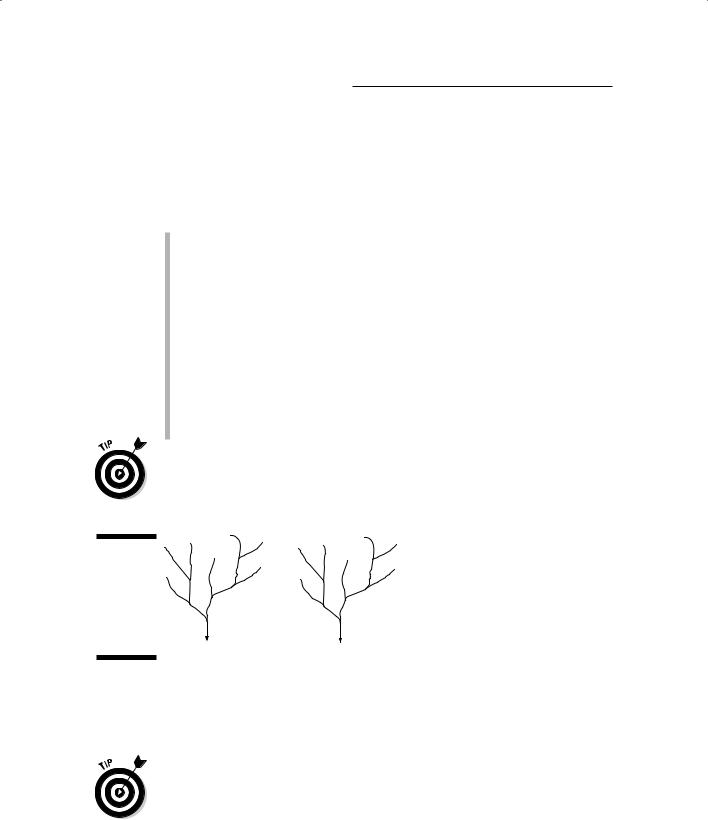
You can calculate stream order in several ways, but the two most common are the Strahler method and the Shreve method. Both of these methods use the exterior link as the first-order stream link and assign these stream tributaries a value of 1 (representing first order), as shown in Figure 14-8:
Strahler method: The most common method. Each new stream order is based on the convergence of two streams that have identical streamorder numbers. When dissimilar stream orders come together, the com-
puter assigns the higher of the two tributaries’ orders to the next stream tributary.
For example, you can use the Strahler method for studies involving sediment movement and stream flow analysis.
Shreve method: Adds the stream orders together to produce the next stream-order number, thus accounting for all possible stream-order combinations. You call these numbers stream magnitudes, rather than orders, because the values aren’t based solely on the ordering.
Ecologists use the Shreve method to reflect how the different stream linkages often result in considerably different ecological conditions.
You can use stream order to define buffer distances because a GIS codes these numbers right into the links themselves.
Figure 14-8: |
1 1 |
|
1 |
1 |
1 |
1 |
1 |
|
|
|
1 |
|
|
||||
The Strahler |
|
1 |
2 |
1 |
1 |
2 |
1 |
|
and Shreve |
1 |
1 |
||||||
2 |
2 |
2 |
|
|
||||
methods of |
|
|
3 |
|
||||
|
2 |
|
4 |
|
||||
determin- |
|
|
|
|
|
|||
ing stream |
|
2 |
|
|
3 |
|
|
|
|
3 |
|
|
7 |
|
|
||
order. |
|
Strahler |
|
|
Shreve |
|
|
|
|
|
|
|
|
|
Some software uses different methods to determine stream ordering — but most of those different methods are really variations on a theme. The
Strahler and Shreve methods are the most common approaches to this type of stream drainage analysis.
Before you start doing work with stream-network analysis, check your software documentation. It usually describes in detail how the methods work and may even provide suggestions for selecting a method.

Chapter 15
Working with Networks
In This Chapter
Figuring out how connected a network is
Working with impedance values
Accounting for directions of movement in linear features
Modeling circuits, turns, and intersections
Putting it all together to model and route traffic
The Earth is filled with linear objects. You can find treelines, fault zones, shorelines, fences, rows of houses — the list goes on. Some linear
objects are special not so much because of what they are, but how they work. These special linear objects are called networks. Networks are collections of connected linear objects such as roads, railroads, or rivers that branch from place to place. They come in different sizes, numbers of branchings, and angular configurations. One classic type of network is the stream network, which allows movement of water along its length. A network that has this movement along its length is called a corridor. This chapter covers the different properties of corridors and shows you how to measure them.
Measuring Connectivity
You can measure connectivity in a network by comparing the number of actual node-to-node links that exist in a given network to the maximum number of nodes that are possible. This measure of connectivity is called the gamma index. Usually, the index ranges from a value of 0 (which indicates no connected links at all) to 1 (where all possible links are connected). Both general and transportation-specific GIS software packages contain algorithms that allow you to calculate the gamma index, which the software records as decimal values.

226 Part IV: Analyzing Geographic Patterns
Recognizing the importance of connectivity
The gamma index gives you a way to determine whether the network is as connected as possible. I once used this index to model the speed at which edge species (species that like to live on the edges of different types of environments) would inhabit a network based on whether that network was poorly, moderately, or highly connected. But most applications of the gamma index relate to human transportation systems.
If you look at a road map of the conterminous United States (the lower 48 states), you may notice that the central portion of the country (the Great Plains) has far fewer road-to-town connections than do the coasts. Most of the coastal areas are highly connected so that each town has many connected links. In other words, the coasts have a gamma index that’s approaching 1. In the Great Plains, many towns aren’t connected directly to some nearby roads, forcing you to take longer routes to get from place to place. Thus the gamma index for road networks in the Great Plains would be closer to 0.
Measuring and using connectivity
A GIS calculates the gamma index by counting all possible connections (links) among all the nodes in the database and then dividing this total (the number of actual links) by the maximum number of possible links. You use the gamma index connectivity figure indirectly when you perform shortestpath analysis (covered in the section “Finding the shortest path,” later in this chapter), but it can also be useful for
Characterizing the loss of shelterbelt networks: Shelterbelt networks are rows of planted, fast growing trees that you use primarily to protect crops from the negative effects of wind. By evaluating the gamma index of shelterbelts, you can begin to plan which regions need the most urgent replantings of trees to replace those that are dead.
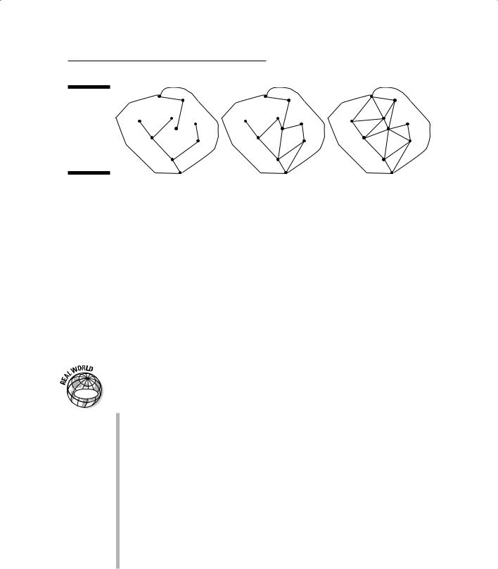
Evaluating increases in road network connections over time: Check out Figure 15-1, where the dots represent towns and the connecting lines represent roads. From left to right, the three networks illustrate how the number of connections among the towns increases while time passes and more roads are built. This increase in connectivity may indicate increased urbanization.
Analyzing the complexity and efficiency of utility networks: Like roads, utility networks provide for flows, but the flows are of electricity, gas, or water. The more connected the utilities are, the more homes they can serve. Some utilities, such as electrical service, often require that substations be appropriately placed to ensure that, if one goes down, others can still provide electricity to all the customers. Analysis to determine appropriate placement is essentially one of connectivity.
Chapter 15: Working with Networks 227
Figure 15-1:
The gamma index increases while connectivity increases.
Working with Impedance Values
When you treat networks as corridors, the movement of fluids, objects, animals, and/or vehicles is your primary concern. For any movement, the nature of the network as a corridor has an impact on how fast things move and in some cases, even whether they move at all. The resistance to movement is called impedance and can be a function of the size of pipeline in a water delivery system, the roughness of dirt or gravel roads, or the number of lanes in highways. The most common use of network impedance is to model street patterns for transportation routing. I use that example in the following sections to show you how network impedance works.
Knowing when your paths are fast or slow
|
Street patterns provide an excellent example of how factors can affect speed |
GIS |
in a network. Speed may increase or decrease for several reasons. Here’s a |
quick list: |
Posted speed limits help determine the maximum travel speeds for streets and highways (sometimes even the minimum speeds).
Fluctuations in traffic density often determine how fast the traffic will move at different times of the day.
Accidents and other unplanned disruptions are bound to slow traffic, especially if lanes are closed off.
Street repairs and changes in road condition often result in changes in traffic flow.
The existence of border checks, sobriety checkpoints, weigh stations, and other regulatory facilities result in slower traffic flow.
Changes in weather, especially the existence of dust storms, rainand hailstorms, blizzards, and sleet storms will often have huge impacts on traffic flow.

228 Part IV: Analyzing Geographic Patterns
Modeling impedance for traffic flow
Given the many factors that affect the movement of flow, especially traffic flow on streets, modeling these changes really improves your ability to know when your grocery deliveries will arrive, how fast a fire engine can get to a fire, the fastest way to get to a particular restaurant for dinner, or the route that you might need to take to pick up your children from their many activities.
When you model impedance, you do have to deal with one complexity — most software gives you many options. And you simply won’t use some of those options because they require that you know much more about your traffic network than you probably do. Ever see those little black traffic counters (they look like rather large power cords) running across your streets from time to time? Traffic engineers and transportation geographers use these counters to determine how much traffic flows past a particular point at any given time. You could easily include this important information in your GIS as impedance data. Other common traffic-flow impedance data include speed limits, stoplights, and stop signs.
Here’s a short list of some of the attributes, or options, that you can put into a GIS impedance layer that you might use for traffic modeling (this list omits data related to turns, which I discuss in the section “Working with Turns and Intersections,” later in this chapter):
Impedance attribute: How long it normally takes to travel a certain distance.
Default cutoff value: The value at which the computer stops searching for a location. You can override or change this value.
Accumulation information: A list of possible attributes that accumulate while distance increases, including costs, students riding a bus, and many more.
Restrictions: Restrictions that you place on the use of links (for example, the permitted types of traffic on portions of your road network). For example, you can choose to force hazardous cargo to use certain streets.
Hierarchy: A set of rules for travel, regardless of how your software determines the impedance values.
These factors (and others that depend on the software you use) are sometimes referred to as the Origin-Destination (OD) matrix. The data for these factors form a separate table. When you use the GIS for transportation modeling, the software compares the network by examining the OD matrix so that it knows the rules to apply and where to apply them. The OD matrix contains several components, including origin, destination, and barrier information.

Chapter 15: Working with Networks 229
By reading the OD matrix, the software knows the ID codes you have placed at strategic locations, how to read the impedances you have linked to those ID codes, and other necessary factors that give you the power to simulate how real traffic flows operate.
Use your knowledge of traffic patterns and impedances to decide which actual values to include in the OD matrix. For example, your matrix entries will reflect attributes such as speed limits for roads, maximum flow capacity for water in a pipeline network, or the amount of electrical resistance you might get from a particular type of wire in an electrical utility network.
Working with One-Way Paths
Impedances, like surface friction values, can be low or high, short distances or long, and even prevent movement entirely. Dead ends, checkpoints, and bridge collapses prevent the movement of travel. You model these impedances by placing no-movement commands at these points. However, you can restrict movement only to one direction by creating unidirectional (or one-way) paths.
Understanding unidirectional paths
In certain situations, travel along a network normally takes place only in a given direction. A fast-moving stream moves rafts in only one direction. Some gate entries allow traffic to move in only one way and out another for control — some gates even place those nasty spikes to rip up your tires if you try to back up. The most common example of a unidirectional path is the one-way street. I focus on that example in the following section because it’s easy to understand and modeled frequently in transportation GIS applications.
Modeling unidirectional paths
If you want to move ambulances, fire engines, or even grocery trucks, you usually look at a map to figure out the best way to get from point A to point B. More than one argument between friends or spouses has begun over disagreements about which path to use. Perhaps you should purchase some GIS software for your friends and loved ones to reduce these disagreements. How would GIS software help? The software is pretty adept at handling the factors that influence travel through a network. One of the most common (and aggravating) situations that street maps don’t often show is the location and direction of one-way streets.
230 Part IV: Analyzing Geographic Patterns
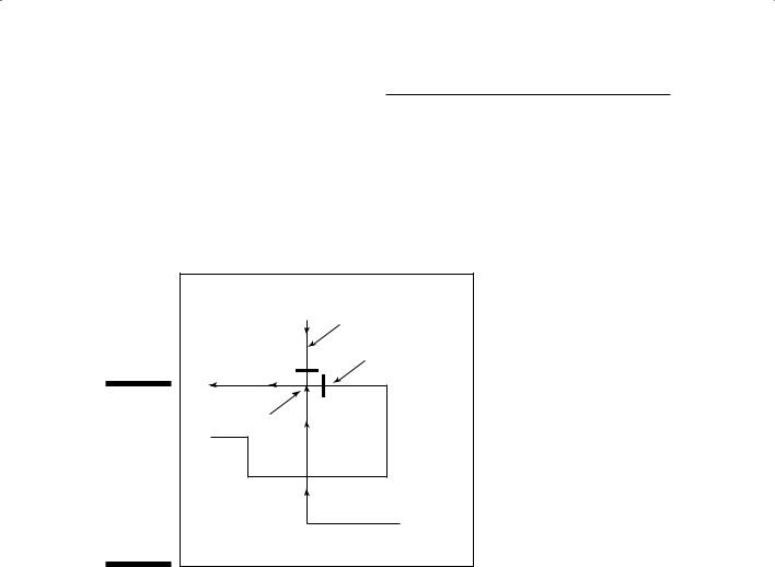
One-way streets are coded in a GIS by including a travel direction restriction in your OD matrix. When the computer tries to model vehicle access to a north-directed one-way street from the south, or even to make turns into it in the opposite direction, the GIS stops the movement and redirects the search to look elsewhere for a path. In essence, the effect is the same as when you put up a barricade across the street that prevents travel in that direction (see Figure 15-2).
|
One-way street |
|
|
One-way street |
|
Figure 15-2: |
|
|
The GIS |
Deflection |
|
software |
Direction of |
|
prevents |
||
movement |
||
movement |
||
|
||
in directions |
|
|
opposite to |
|
|
the direction |
|
|
of one-way |
|
|
streets. |
|
Characterizing Circuitry
A network’s complexity is partly measured by the numbers of links it has compared to the maximum number it could have (the gamma index). One other factor both characterizes the complexity of a network and adds to the robustness of traffic modeling capabilities. That characteristic, called circuitry, is based on the idea of closed loops. Closed loops allow moving objects, fluids, and so forth to travel alternate routes when moving along a network (see Figure 15-3). The following sections show how closed loops work.
Knowing when lines create circuits
If you’re modeling streams, you may encounter a location where a stream splits around an island and can move in two different directions. In forests, some wildlife takes advantage of circuits to avoid predators because the prey