GIS For Dummies

Chapter 12: Measuring Distance 191

Establishing Relative Measurement

Sometimes, you don’t need to know the exact distance from a reference point to a feature; you just need to know whether that feature is close to or far from the reference point. In some cases, a feature might actually be touching the reference point, a position that’s called adjacency.

Relative measurement is the type of information you need every day. If you ask about the distance to something, you don’t always expect, nor even want, a precise answer. For example, say you’re in a new town and stop to ask directions — “How far am I from the courthouse?” You receive the answer, “It’s about 766 meters east south east as the crow flies.” This answer gives you an idea of where it is and how far, but you were really looking for something like, “It’s just a short drive down this street and around the corner.” In other words, you just wanted to know whether you were close or whether you had to drive for quite some time.

You can use relative measures in many ways:

Selecting among different locations

Deciding whether you have time to get someplace

Knowing whether features such as towns are going to interact with each other

Determining whether you can find sufficient beachfront property for a resort

Adjacency and nearness

When your reference point is so close to a feature that the distance between them is essentially zero, you call that distance adjacency. The distance measure for adjacency involves how many features are at a distance of zero from your reference point.

Because relative measurement requires a starting point, you can easily determine whether something is near or far by creating distance buffers based

on your definition of near or far. Current GIS technology can easily measure distance, but it can’t make decisions about what you consider near or far for a given application. Suppose that you want to know which parcels of land are near (within a given specified distance of) a lake. You follow these basic steps to define near as within a quarter mile of the lake:

Chapter 12: Measuring Distance 193

Containment and surroundedness

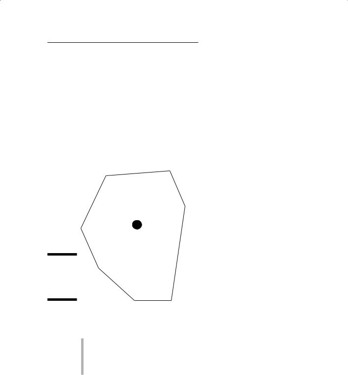
You generally think of measuring distance from one thing to another thing. When your reference point is inside a polygon, its distance from the edge of that polygon is measured inward toward the reference point rather than outward toward other features. This idea is called containment. Containment can help you figure out what features are inside other features.

To measure containment, the GIS essentially measures a distance inward from the edge vertices (the corners) of a polygon or area feature, determining whether the X and Y coordinates of your object are all contained within

the limits of the X and Y coordinates of the polygon that you examine (see Figure 12-7).

Point Object

Figure 12-7:

A point object contained in a polygon.

Knowing whether an object is contained in a polygon can help you answer these kinds of questions:

Does the property I’m interested in fall within a certain school district?

Does a particular wildlife species live in a certain habitat type?

Do I live inside a 100-year flood zone?

Which voting district do I live in?

To answer questions like these (for example, about voting district), you usually let the program compare the data from two different maps (for example, a street map and a precinct map) because both kinds of data (street addresses and precinct boundaries) don’t appear on the same map. Still, to

194 Part IV: Analyzing Geographic Patterns

determine whether the distance would be inward (contained) or outward (not contained), you use the same calculations that you do for a single map analysis because the software essentially compares the X and Y coordinates of the points on one map (the street addresses) to the polygon coordinates (the precinct boundaries) on the other map.

You can assume that a point object exists either inside or outside a given polygon because it has zero dimensions. If you ask whether a line feature (such as a highway) is in a polygon (such as your state) or another polygonal feature (such as a park) is in a polygon (such as your city), you add dimensionality that complicates the answer. You can have a situation in which part of a line or polygon is within another polygon. GIS can help you determine whether these objects are only partly in a given polygon by simply comparing the locations where the two sets of features intersect.

Measuring Functional Distance

Functional distance is a measure of space based on how that space is used, rather than its absolute measurement. Functional distance recognizes that you don’t always want to know exactly how near or how far, but rather what traveling that distance might cost you in time, money, calories, or even just emotional distress. Simply put, you use a different measuring device than for absolute measurement. Say that you ask the question, “How far is it to the interstate highway from here?” You might get a functional-distance answer of, “Oh, not far! Maybe a couple of minutes.”

You can base functional distance on these kinds of factors:

Expenditure of fuel, based on how long it takes to travel a distance

How much a trip costs

How much wear and tear you put on your vehicle

How much stress the trip puts on the travelers

These factors can influence functional distance measurements:

The ruggedness of the terrain

Whether the roads are well maintained

The amount and direction of wind

You can find as many functions of geographic space as you can find potential users. The following sections describe various forms of functional distance.

Chapter 12: Measuring Distance 195

Anisotropy (whew!) — non-uniformity

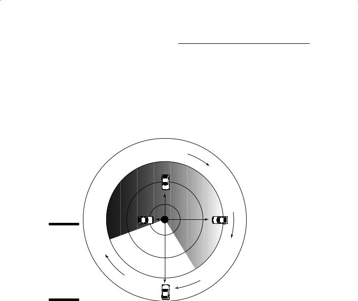
GIS sometimes gives you a chance to impress your friends because you know all these cool-sounding words that they’ve never heard. One such word is anisotropy, which is the opposite of isotropy. Isotropy is the property of a totally smooth surface that has no paths, bumps, wrinkles, vegetation, or obstructions of any sort. If you find an isotropic surface, let me know because it’s really just a theoretical property. Isotropy doesn’t exist in nature, but it does give you a standard against which you can compare all your anisotropic surfaces.

A perfectly isotropic surface that has no obstructions and no slopes, and a totally smooth surface produces a situation in which you can travel outward from its center in any direction and end up at the same distance from the center as you would if you’d gone in any other direction. It’s sort of like a series of concentric circles in which the circles show distance traveled at selected times.

When you want to measure distances from a point or area to all other locations throughout a surface, knowing that the surface isn’t uniform (meaning not isotropic), the idea of anisotropic surfaces comes in. The roughness of the surface is a measure of its departure from the perfect isotropic surface. The rougher the surface, the more likely it is to produce friction (resistance to movement), as shown in Figure 12-8. The steepness, type of surface, or stability of the subsurface can cause varying degrees of friction. Factors such as the time of day, direction of travel (uphill or downhill), and how long the traveler has been traveling also influence non-uniformity.

Accounting for physical parameters

The most common factors associated with impeding travel are physical:

Slope: The steeper the uphill slope, the more friction you experience. Think about how driving uphill into the mountains both puts a strain on your engine and draws heavily on the old gas tank. This same friction impedes bicyclists, hikers, and even wildlife.

Type of surface: You can much more easily traverse smooth concrete than soft sand; you can walk along a well-trodden hard path more easily than saturated ground or mud.

Surface features: The surface itself has the ability to support features that contribute to the impedance or friction value of the surface — such as vegetation. Think how much more easily you can travel along a soft grassy surface than along one that has thickets or trees.

Chapter 12: Measuring Distance 197

Researchers have established a few measurable friction surfaces as standards for some physical features under selected situations. One of these, the Universal Soil Loss Equation, models the loss of soil during rain events. Within that equation, you need to assign a value to a surface type based on the average soil erosion factor for each soil. You then plug these generalized numbers into the equation and get a calculated estimate of how much soil will erode from a surface based on the surface type.

For GIS, the process of modeling friction surfaces is much the same as using the Universal Soil Loss Equation. (In fact, soil scientists and soil geographers have used the Universal Soil Loss Equation in GIS modeling.) The GIS modeler must encode any impedance to movement into a special map layer, often called a friction layer. The greater the friction value, whatever it’s based on, the higher the value stored in the friction map.

In theory, you can quantify friction easily: big friction = big numbers, little friction = little numbers, no friction = zero. But, in reality, the process is a bit more complex than that. Ask yourself how you might give friction values to some of the following:

Difficulty of crossing a stream

Resistance of thickets for hiking

Resistance of forests to deer movement

The impact of fatigue on walking uphill

The expenditure in calories of a cougar traversing a rugged mountain

The impact of temperature on the movement of disease

And beyond these physical factors, imagine trying to model the impact of scenery on the apparent time of travel. How do you put in numbers friction values that have no standards and no measurements? You can use a scalar level of geographic measurement, in which you establish the scale of measurement. If you use a scale of 0 to 10, you probably know at least two values of your scale — 0 and 10. The 0 value indicates a condition that includes no resistance to travel at all, and 10 indicates that no movement can take place.

You need to decide where, within that range, other friction values might fall — by using experience, expert opinion, some measurements, surveys, or any number of different ways to gather some basic information. Unfortunately, you’re stuck with a combination of guesses, experience, opinion, and luck. But although little may be known about friction surfaces, you can usually figure out the maximum (a barrier) and minimum (frictionless) values that allow you to place the upper and lower limits on your scale.

198 Part IV: Analyzing Geographic Patterns

Calculating the functional distance

No matter how you define your numbers, your friction map must interact with another map layer that you use to find distances to and from places. Raster data models always work best for this kind of layer interaction. Figure 12-9 shows a raster data model. When you move from cell to cell in this data model without accounting for friction, you simply add the distance of the grid cells (1 width for orthogonal and 1.414 for diagonal, see the earlier section “Measuring distances in grid cells”).

After you take friction into account, the computer must add not just the distance, but also the friction value before it can actually continue to calculate distance for the next cell. So, the higher the friction number, the more the computer has to add to the cumulative distance value before it graphically moves to the next grid cell.

1 + 1 + 3 (friction)

Chapter 13

Working with Statistical Surfaces

In This Chapter

Knowing what makes surfaces tick

Working with the various types of statistical surfaces

Estimating values with interpolation

When most folks hear the term surface, they think of the physical surface of the ground beneath their feet. Paper maps that show topog-

raphy use elevation lines, and some globes actually have raised surfaces to indicate mountain ranges. With GIS, surface means much more than the physical topography. You can map and analyze many different statistical

surfaces, which include features such as population density, crime rates, and cost of living. This chapter shows you the ins and outs of statistical surfaces, beginning with an overview of just what makes them tick.

Examining the Character

of Statistical Surfaces

In GIS, the definition of surface is much broader than simply the physical surface of the land, or topographic surface. Surfaces can relate to other factors of the physical environment that help to create non-physical, or statistical, factors.

Non-topographic statistical surfaces come in two general forms — those relating to the physical environment and those relating to the human environment. This breakdown doesn’t have any intrinsic value; it just provides a simple way to categorize non-topographic statistical surfaces. In the following sections, I refer to only those human environmental factors that relate to social and economic activities because these factors are easier to understand than the less tangible surfaces (such as those related to beliefs or attitudes, for example, whether people think economic conditions are improving) that occasionally appear in more obscure applications.

200 Part IV: Analyzing Geographic Patterns

Here are examples of the two general forms of statistical surfaces:

Physical environment: The most obvious physical statistical surface is topography, but many others are nearly as common and quite useful. Many physical maps relate to subsurface phenomena such as depth to bedrock, depth to groundwater, thickness of rock formations, depth to the ocean floor, and many others. Other physical surfaces are more

closely related to climate and weather phenomena, such as temperature, barometric pressure, and precipitation.

Human environment: Think about human environment in terms of socio-economic data. These data deal with people — their numbers, ages, races, education levels, and incomes — and with factors that affect people, such as cost, home values, and taxes. Socio-economic data can even represent disease, crime, attitudes, and belief systems. Because socio-economic data relate to geographic features that don’t normally occur everywhere (that aren’t continuous), analyzing such data often requires that you suspend disbelief (pretend that what really doesn’t occur everywhere actually does) and treat them as proper, formal statistical surfaces.

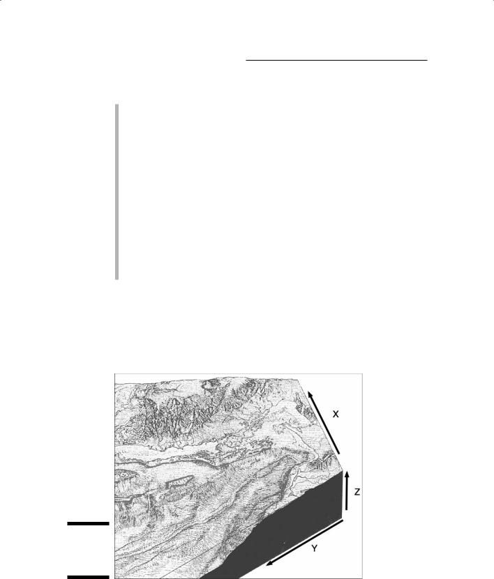
All these factors and thousands more involve the measurement and mapping of values, each of which has a pair of X and Y coordinates (for location) and a third value — the Z value — which describes the surface. You can turn the values for each physical or human environment factor into a map of the surface that shows the highs and lows in Z value in different places (as illustrated in Figure 13-1).

Figure 13-1:

X, Y, and Z values of a surface.