

GIS For Dummies
.pdfChapter 5: Understanding the GIS Data Models |
91 |
|
|
|
|
|
1 |
|
|
1 |
X |
Y |
Z |
|
|
Figure 5-11: |
2 |
X |
Y |
Z |
|
|
3 |
X |
Y |
Z |
1 |
||
A 4 |
X |
Y |
Z |
|||
5 |
||||||
Triangulated |
5 |
X |
Y |
Z |
||
Irregular |
6 |
X |
Y |
Z |
8 |
|
Network |
7 |
X |
Y |
Z |
|
|
8 |
X |
Y |
Z |
|
||
model. |
|
Point file |
|
|||
|
|
8 |
||||
|
|
|
|
|
||
|
2 |
|
|
|
Vertices |
Neighboring |
|
|
|
||
3 |
|
triangles |
|
|
|
2 |
4 |
4 |
|
1 |
1 |
6 |
5 |
2 |
8 |
X |
|
2 |
1 |
4 |
6 |
1 |
3 |
6 |
|||
6 |
|
|
|
3 |
1 |
2 |
4 |
X |
4 |
2 |
|
|
|
3 |
|||||||
6 |
|
5 |
4 |
2 |
3 |
4 |
3 |
X |
5 |
|
|
|
|||||||||
|
|
5 |
4 |
3 |
7 |
4 |
X |
6 |
||
|
|
|
|
|||||||
7 |
|
|
|
6 |
6 |
4 |
7 |
2 |
5 |
7 |
|
|
|
|
7 |
6 |
7 |
8 |
6 |
X |
8 |
|
7 |
|
|
8 |
5 |
6 |
8 |
1 |
7 |
X |
|
|
|
|
|
|
Triangle file |
|
|
||
|
|
|
|
|
|
|
|
|
||
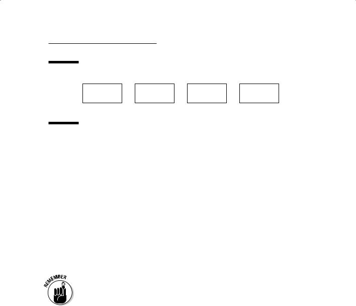
TINs are topological data models, just like DIME and TIGER models presented earlier in this chapter, but they’re specifically designed to incorporate the Z value component, whether it’s topography or economic data. Like in other topological data models, the TIN data model contains explicit information about which features are related spatially to others.
The TIN model, shown in Figure 5-11, is pretty close to the model you see in Figure 5-7. Each model has a table of point values, and each has a set of
polygons and links. In the case of the TIN model, the polygons are always triangles, and each triangle’s vertices define it. The Triangle File table in the TIN model is much like the polygon table in Figure 5-7. Specifically, the Triangle File table shows
The vertices that make up each triangular facet (the first three columns)
The neighboring polygons (the second three columns)
The Point File table is different in the TIN topological model, as compared to the chain table in Figures 5-8 and 5-9, because it also contains the elevation
(Z) value for each.
The TIN model has some definite positive features:
It’s incorporated in many vector GIS packages, so it can be used immediately for surface representation.
You can easily convert it to matrix models, such as the digital elevation model (DEM).
It allows for interpolation of missing Z values by using a wide variety of algorithms.
You can make cross-sectional profiles of terrain and perform many advanced functions related to topography.

92 |
Part II: Geography Goes Digital |

Chapter 6
Keeping Track of Data
Descriptions
In This Chapter
Understanding how simple graphics programs store descriptions
Working with database management systems
Using object-oriented systems to provide more geographic reality
No matter what type of geographic setting or scales of geographic data you use in GIS, you need to link the graphics with meaningful descrip-
tive data. When you perform geographic analysis, you search, manipulate, compare, and analyze this data. Every GIS software package must manage descriptive data and link them to their respective objects on the map.
Without this capability, your GIS is nothing more than a digital picture, and you may as well work with a paper map.
You can find many programs that contain both graphic elements and descriptions, such as graphics drawing packages, complex drafting and design programs, facilities management packages, and computer-assisted mapping programs. These programs aren’t, technically, geographic information systems, but they may possess some of the functionality of GIS and definitely link data descriptions with graphics in a similar way. Getting a feel for how these simpler systems handle data-to-graphics linking can help you understand how more complex GIS do the same thing. Consequently, this understanding can help you select the software that meets your needs.
In this chapter, I describe how simple software systems store descriptive data and link them with the appropriate graphics. I tell you what these various systems do well (for example, computer-assisted cartography programs do a great job of storing geographic information and outputting maps) so that you can have an idea of how well the software can handle the analytical tasks that you have in mind. Who knows? You may decide that one of these simple systems fits your needs just as well as a full-blown GIS.

94 |
Part II: Geography Goes Digital |
Knowing the Simple Systems for Tracking Descriptions
There are many kinds of software for dealing with different forms of graphical data like house plans, satellite images, and maps. In fact, development of these innovative programs took place simultaneously and for different purposes, as follows:
For analyzing satellite images: People needed ways to manipulate electronic images gathered remotely from satellites orbiting the Earth. They began developing raster manipulation (image processing) software to analyze those digital images.
For basic mapping of Earth features: Other folks were interested in mapping Earth’s features, so they developed raster and vector mapping software.
For drafting and design work: And people involved in drafting complex buildings, machinery, and so on created computer-aided design (CAD) and drafting software.
You can still find each type of software in the preceding list available today in one form or another. Each software type has its specific application, and various developers are collaborating across applications to the mutual benefit
of all the different types of users. Because of the convergence of the different tasks, the properties of CAD programs have changed from their original form to a more GIS-like software. The descriptions in the following sections are somewhat simplistic, reflecting the original purpose and design of each type of software. When you consider your options, pay attention to the original conceptual design, as well as the capabilities that the software possesses in its current state.
Understanding computer-assisted cartography
Like GIS, computer-assisted cartography (CAC) was created to store, edit, and output maps of the Earth and — crazy as this sounds — other planets. CAC doesn’t have the analysis capability that’s at the heart of GIS, however. CAC is a straightforward process that moves from input to storage, retrieval, editing, and finally, output (see Figure 6-1). A CAC system just needs to store the attributes, or descriptive data, and have labels attached to the attributes so that those descriptive labels can be applied during output.
Chapter 6: Keeping Track of Data Descriptions |
95 |
Figure 6-1:
The computer-
assisted Input  Storage / Edit
  Retrieve
  Output cartography
linear process.
This simple system of linking the graphics to individual attributes makes CAC an efficient approach to store and output maps that have symbols and legends, but it limits both the amount of attribute data you can store for each entity and your ability to manipulate it. The usual way that such systems store attributes is as a list in which each attribute (description) is associated with individual graphic objects. For example, a graphic polygon might have the name Mirror Lake associated with it in the attribute list. Each map has its own geographic elements, called entities, and its own attributes. CAC doesn’t allow maps to share either their entities or their attributes with other maps in the same database. As a result, you can’t use CAC to overlay one map on another or combine their data in other ways.
CAC software allows you to translate input coordinates (such as digitizer inches) into scaled map data. You can also use CAC to convert from flat, planar coordinates to geographic coordinates, which allows you to convert map projections to land-based coordinate systems and vice versa. If your purpose is to input, archive, update, and output maps, CAC is the system for you.
If you plan to use a system only for map production, computer-assisted cartographic systems are both more efficient and more cost-effective than the more complex GIS software. CAC doesn’t have the analysis capability that’s at the heart of GIS, however.
Using computer-aided design
Like computer-assisted cartography, computer-aided design (CAD) isn’t intended to manipulate or analyze cartographic data. In fact, CAD isn’t intended to work with cartographic data at all — but it can. CAD systems — which are designed to store complex drawings in layers — store attribute (descriptive) data as linked lists tied explicitly to the drawing’s components (the entities) on a layer-by-layer basis. This layer-by-layer division means that the data are not shared from one layer to another.

96 |
Part II: Geography Goes Digital |
CAD is capable of performing visual overlay because of its inherent layered data model — unlike CAC, CAD is structured to store multiple data descriptions that apply to the same entity. Many times, the graphical overlay operations produce graphics that help you visualize the data, but they don’t create new data from the various combinations of layers. GIS is designed to do so, however, which allows you to compare one map pattern to another.
Another major difference between CAC and CAD is that, generally, CAD doesn’t include much capability to change projection or coordinate systems. You can’t convert from one form of map projection to another or change from one coordinate system to another, for example.
One nice feature of CAD is that a standardized exportable version of the typical .dwg file (a common CAD drawing file), called the drawing exchange format (.dxf), is often easily translated from CAD to both CAC and GIS software. In fact, many people use CAD software for input because they find the user interface for the input task easier to use than the GIS interface.
Exploring raster systems
The basic raster system method of handling attribute data is to store them as a set of ASCII characters (meaning letters and numbers), usually numbers. Each grid cell has a single numeric code associated with it. In most raster systems, the numbers are whole numbers. The code, in turn, is linked to a legend description (the names of the categories) and to a symbol set (the colors or shades used to represent the categories) for final display.
Storing attribute data in a raster system
Storing attribute data in a raster (grid) system requires that you store the value of each individual square based on its location in the sequence of grid cells. So if you are using a grid system that starts in the upper left and moves to the right, the first value you store would be for upper-leftmost grid cell. You assign the numbers (codes) based on how you define the attributes from the start. While the values may be actual measurements for things like elevation or slope, you may also assign numbers to represent categories, such as 0 for water, and 6 for agriculture, and you make these decisions before you start putting the numbers in the database.
Suppose that you want to use the number 6 to represent agriculture. To do so, you place the value (code number) 6 in the first column, first row. It turns out the next cell in sequence is also agriculture, so you put the number 6 in the second column, first row. If you know that the third grid cell over (the third column) in the first row is water and you want to use the code of 0 for that, you just enter 0 in that grid cell (third column, first row).
Chapter 6: Keeping Track of Data Descriptions |
97 |
You don’t need to input these grid cell values manually anymore, but this example gives you an idea of how a typical GIS user would sequence them. You know the location of each grid cell of each type because you placed them where they needed to be, and you can easily retrieve the categories that you want based on the numbers you assigned.
When your GIS represents topography (the depiction of land surfaces), it doesn’t have to use whole numbers. Some systems use only whole numbers to represent the Z value, but that approach limits the accuracy of the surface data. Most modern GIS software allows for the more accurate use of rational numbers expressed as decimals. The more accurate the numbers, the better are the results of your analyses. Check out Chapter 14 for more about working with topographic surfaces.
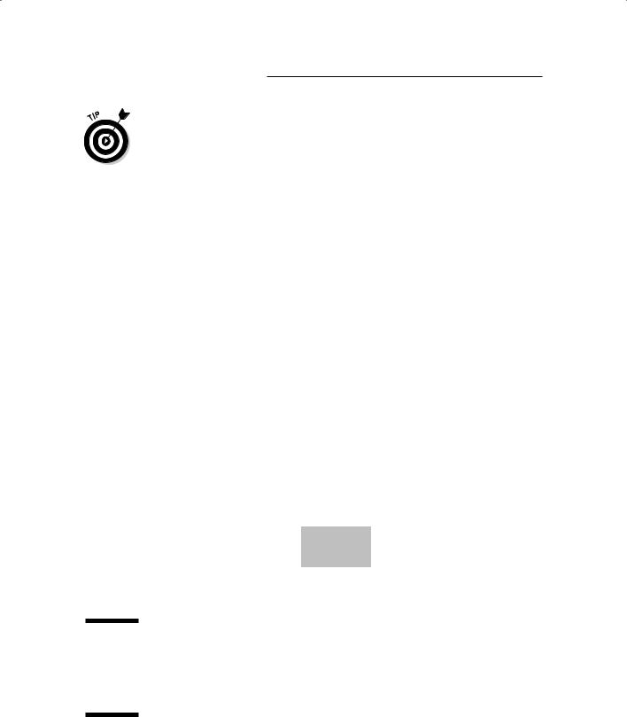
Map modeling with grid systems
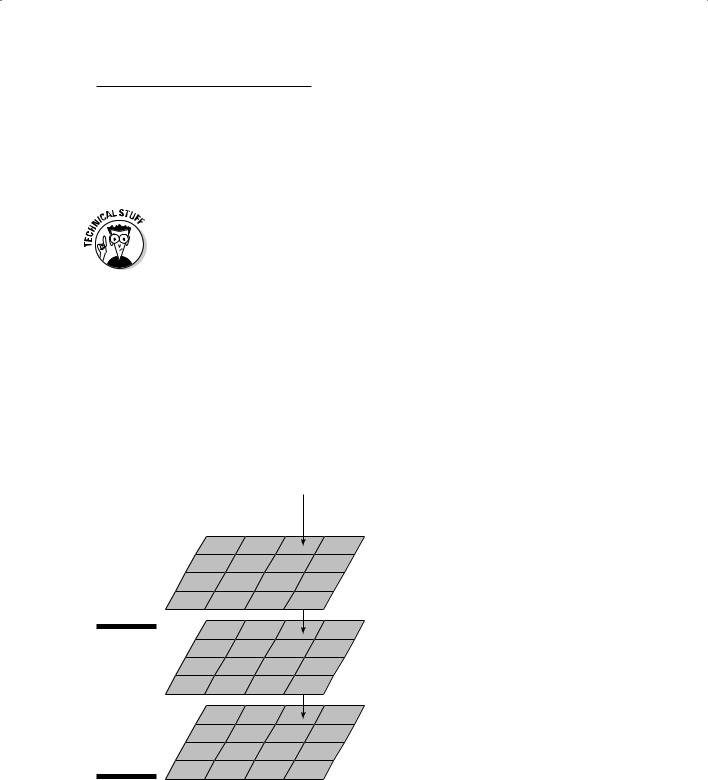
Although the raster method is pretty simple to understand, you can’t beat it when you want to store, analyze, and compare map attributes. Each grid cell for each grid layer is a uniform size and shape. Each grid layer is composed of identical numbers of columns and rows, in which each respective grid cell is positioned in exactly the same geographic (column and row) space (see Figure 6-2). In other words, a grid cell in the upper-left corner of one map layer is in exactly the same position as any other upper-left-corner grid cell for any other map layer.
Figure 6-2:
In raster storage, you can compare each map
layer to every other map layer.

98 |
Part II: Geography Goes Digital |
Because each grid cell contains attribute data, you can easily retrieve the data and compare it to its respective grid cell in another map layer. You use this property when you compare one map to another (especially when you use the Map Analysis Package, or MAP, data model, which I cover in Chapter 5). In Chapter 17, I show you how this characteristic was used to create a complete GIS modeling language called map algebra.
Because raster grid cells are uniform in size and identically placed from one map layer to another, you may find them especially useful when you must perform map overlay operations for map analysis. Also, because the raster model is so simple, it makes map overlay faster than in vector systems, which usually have more complicated data structures (see the section “Managing data in Vector GIS” for more about these structures).
Working with Tables and Database Management Systems
Database management systems (DBMS) were created to manage data. As glib (and completely obvious) as that may sound, the idea is significant because DBMS weren’t originally designed to manage all types of data, and specifically, not spatial data. The original database management system was a separate technology that had a different clientele in mind. In the early development of GIS, the DBMS stored attribute data, and the graphic data were stored elsewhere.
|
Environmental Systems Research Institute (ESRI) first fully implemented the link |
|
|
between graphics and descriptions stored in a database management system in |
|
GIS |
its premier product called ArcInfo. The name is rather telling. Arc is the portion |
|
of the software suite that deals with the graphics, and Info is an existing data- |
||
|
||
|
base management system that’s linked to Arc so that changes in entities (the |
|
|
graphics) are reflected in changes in attributes (the data) and vice versa. |
Structuring simple relational data
At the heart of these systems is the database management system itself. These systems are called relational database management systems (RDBMS) because of their ability to form associations (relations) among the various data they contain. The data you search are contained in rows called tuples (pronounced tooples) and are grouped with corresponding rows called relations. These groupings of rows are called relations because the information they contain is related. Specifically, each piece of data (column) in a single row is related to that column’s data in the other rows because each row contains identical categories that can be compared to one another. Each column represents an attribute — such as a parcel ID or house number for an address book — that’s common to each tuple in the entire relation.

Chapter 6: Keeping Track of Data Descriptions |
99 |
As an example, Figure 6-3 shows a land-use table. Each row contains a different Parcel-ID so that all the information in that row belongs to that one person. Each column contains a unique type of information, and each individual item is linked to the name in its respective row. The relationship among the pieces of data in a single row is a tuple. Collectively, you call this a table of relations.
|
|
PARCEL-ID |
LUCODE |
LANDUSE |
STATUS |
OWNER |
PRICE |
|
|
F2300223 |
010002 |
row crop |
active |
Sylvia Porter |
$1,000 |
|
|
|
|
|
|
|
|
|
|
F4139992 |
020001 |
orchard |
dormant |
Robert Orange |
$1,500 |
Figure 6-3: |
|
||||||
|
|
|
|
|
|
|
|
A relational |
|
F2889881 |
030001 |
rangeland |
active |
Joseph Barney |
$650 |
database |
|
||||||
|
|
|
|
|
|
|
|
|
F9887632 |
010002 |
row crop |
active |
Sylvia Porter |
$1,200 |
|
manage- |
|
||||||
ment system |
|
|
|
|
|
|
|
|
F0998944 |
010004 |
garden farm |
active |
Alice Stalk |
$2,000 |
|
(RDBMS) |
|
||||||
|
|
|
|
|
|
|
|
table. |
|
F7966501 |
010002 |
row crop |
dormant |
Jordan Waits |
$1,100 |
|
|
||||||
|
|
|
|
|
|
|
|
Each table operates like a set (for example, a set of land-parcel owners, together with the parcels they own and additional information about those parcels). These tables follow certain rules to store and, more importantly, retrieve data from these sets, including the following critical rules:
A table can’t have duplicate rows. Imagine, for example, if a row represented your land holdings. You need to have the information for each parcel included only once. Each row in a table should represent a unique entry.
A table must be searchable. Each row of data is unique, so to find a unique entry, you can use one or more columns (containing a specific type of data) to search the rows. You could, for example, search by owner’s last name, an ID number, or a land-use type. You can much more easily use a single column to search the rows of data if you set up the table so that you know which column you want to use. This preferred column — often the first column and the one you most often use to do your search — is called the primary key.
To successfully find the right data, though, you need to make sure that the primary key has a value that you can search. Missing values in the primary key could result in duplicate rows of data (that’s a problem because the computer program has no way to determine which row it should be looking at). And even worse, if the primary key has no value, there is no way to connect to the remaining data in the row. It would be like having an address book that was missing names.
100 Part II: Geography Goes Digital
A good rule for database management systems is to make your tables very simple so that you know exactly what you’re going to search, what your primary key is, and what you expect to find. Focus on one or two queries that you want to make for each table. Ask yourself, “What questions do I want to be able to ask about the data in this table?”
Getting more complex with relational joins
Figure 6-4:
Arelational join links
tables by
acommon column.
Simple databases, although easier to understand and control than more complex ones, aren’t going to be of any use to you if they don’t give you access to the large, complex datasets like the ones that you encounter in most GIS operations. But a relational join can help by allowing you to segment your database into nice bite-sized chunks that you can compare later (as shown in Figure 6-4). The relational join is a linking mechanism that allows you to match data from one table to another. You can link as many tables as you like
by matching a column (the primary key) in one table to another column in the second table. The linked column in the second table is called a foreign key.
LUCODE |
LANDUSE |
STATUS |
OWNER |
PRICE |
10002 |
row crop |
active |
Sylvia Porter |
$1,000 |
|
|
|
|
|
20001 |
orchard |
dormant |
Robert Orange |
$1,500 |
|
|
|
|
|
30001 |
rangeland |
active |
Joseph Barney |
$650 |
|
|
|
|
|
10002 |
row crop |
active |
Dabney Porter |
$1,200 |
|
|
|
|
|
10004 |
garden farm |
active |
Alice Stalk |
$2,000 |
|
|
|
|
|
10002 |
row crop |
dormant |
Jordan Waits |
$1,100 |
|
|
|
|
|
COMMON
KEY
OWNER |
STREET |
CITY |
Phone |
Sylvia Porter |
401 Main St. |
Aggieland |
555-5542 |
|
|
|
|
Robert Orange |
1410 Oak Ave. |
Aggieland |
555-0024 |
|
|
|
|
Joseph Barney |
12 Eagle Ct. |
Pottsville |
555-4429 |
|
|
|
|
Dabney Porter |
401 Main St. |
Aggieland |
555-5542 |
|
|
|
|
Alice Stalk |
222 W. Elm |
Aggieland |
555-2218 |
|
|
|
|
Jordan Waits |
1002 E.Pine |
Aggieland |
555-0991 |
|
|
|
|