

GIS For Dummies
.pdfChapter 5: Understanding the GIS Data Models |
81 |
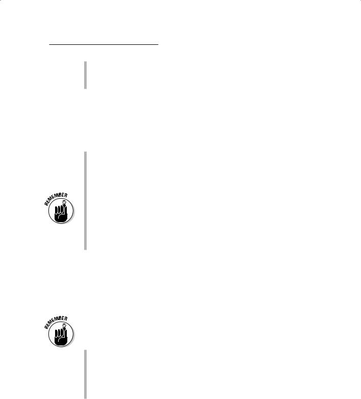
Figure 5-5:
The spaghetti vector data model is a one-to-one translation of the graphics into the computer.
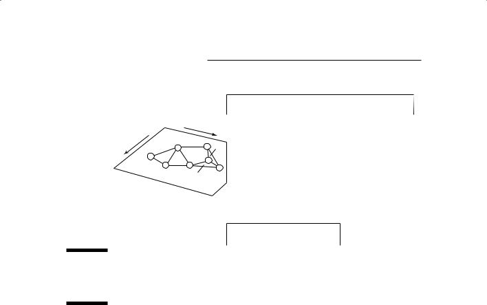
Figure 5-6:
The shapefile data model supports these geometric shapes, among others.
Analog map
|
|
|
|
|
16 |
|
|
|
|
25 |
26 |
|
|||
|
|
x 5 |
|
|
|
||
|
|
|
|
|
|
|
Digital map in |
|
|
|
|
|
16 |
Cartesian Coordinates |
|
|
|
|
|
|
(Data model) |
||
|
|
25 |
26 |
||||
|
|
|
|||||
|
|
x 5 |
|
|
|
||
|
|
|
|
|
|
Data Structure |
|
|
Feature |
|
Number |
|
Location |
|
|
|
Point |
|
5 |
|
x,y (single pair) |
|
|
|
Line |
|
16 |
|
(string of x,y coordinate pairs) |
||
|
Polygon |
|
25 |
|
(closed loop of x,y coordinate pairs where first and last pair are the same) |
||
|
|
|
26 |
|
(closed loop sharing coordinates with adjacent polygons to form a data structure) |
||
|
|
|
|
|
|
||
|
Value |
Shape type |
|
|
|
||
|
|
|
|
|
|
||
|
0 |
Null shape |
|
|
|
||
|
|
|
|
|
|
||
|
1 |
Point |
|
|
|
||
|
|
|
|
|
|
||
|
3 |
PolyLine |
|
|
|
||
|
|
|
|
|
|
||
|
5 |
Polygon |
|
|
|
||
|
|
|
|
|
|
||
|
8 |
MultiPoint |
|
|
|
||
|
|
|
|
|
|
||
|
11 |
PointZ |
|
|
|
||
|
|
|
|
|
|
||
|
13 |
PolyLineZ |
|
|
|
||
|
|
|
|
|
|
||
|
15 |
PolygonZ |
|
|
|
||
|
|
|
|
|
|
||
|
18 |
MultiPointZ |
|
|
|
||
|
|
|
|
|
|
||
|
21 |
PointM |
|
|
|
||
|
|
|
|
|
|
||
|
23 |
PolyLineM |
|
|
|
||
|
|
|
|
|
|
||
|
25 |
PolygonM |
|
|
|
||
|
|
|
|
|
|
||
|
28 |
MultiPointM |
|
|
|
||
|
|
|
|
|
|
||
|
31 |
MultiPatch |
|
|
|
||
|
|
|
|
|
|
|
|
Complex forms of vector representation
Despite its robustness and elegance, the shapefile (see the preceding section) lacks one thing that many high-end modelers demand — the ability to see spatial relationships. This characteristic, called topology (which I define more specifically in the next section), allows the GIS software to recognize

82 |
Part II: Geography Goes Digital |
and convey some basic spatial relationships that humans express by using an English language construct called the prepositional phrase. (Don’t worry. You don’t have to diagram sentences.)
In everyday language, you use many prepositional phrases that describe the spatial relationships you encounter. For example, you may live “outside a town,” “next to your neighbor,” and “within the county.” You travel roads that go “through forests,” “along rail lines,” and “over hills.” The data models discussed in the section “Simple forms of vector representation,” earlier in this chapter, don’t have these relationships (known as topological relationships) explicitly coded. You need to incorporate the mathematics of these relationships — the topology — into the data model so that you don’t have to calculate these spatial relationships each time you want to analyze something.
Using the mathematics of neighborhood
When you look at a map, you can easily see where everything represented on the map is relative to everything else on that map. For example, when you look at a map of your own neighborhood, you get an instant view of that neighborhood. You can see shortcuts, recognize which places are close to your house and which are far from your school, determine what’s on each side of your street, and know which streets are connected to each other and which aren’t. To replicate this powerful property of the human brain inside the computer, computer scientists employ a branch of mathematics called
topology that studies the positions and relative locations of geometric figures. I like to call it the “mathematics of neighborhood” because it allows the computer to understand how a neighborhood works (including what features are located there, where they are relative to each other, and how to find them).
Because computers can’t reason or look around at their neighborhoods, you have to tell them everything. And so you explain
Each line you create is linked to other lines. If the computer understands these connections, you can move from one link to another, just like you’d drive your car from one street to another.
The classifications of nearby areas. Say that on the left side of a line (perhaps your street) is a polygon (a parcel of land) that’s agricultural, and on your right side is a single-family residential parcel.
The U.S. Bureau of the Census needed computers that understood the connections and classifications used in its work. This need led the bureau to develop two of the more well-known topological data models — the Dual Independent Map Encoding (DIME) and subsequent Topologically Integrated Geographical Encoding and Referencing (TIGER) models (discussed in the following section).
Figure 5-7 shows a generic topological vector model. All the others, including commercial ones, are based on this model, with minor variations. The left side of the figure shows several points, lines, and polygons, all of which are numbered:
Chapter 5: Understanding the GIS Data Models |
83 |
Points: The numbers that have circles around them
Lines: The numbers that interrupt the lines
Polygons: The numbers inside the polygons
These numbers are essential because they allow the computer to know which part you’re referring to when you want to compare the relative locations of all the points, lines, and polygons.
The table at the top of Figure 5-7 contains information about the spatial relationships (the topology) of the points, lines (links), and polygons:
Link #: Lists all the links in the figure, numbered 1 through 11.
Right and left polygons: Tell you how the links are related to the polygons on either side of them. This is the contiguity property of topology, which identifies the polygon on either side of any given line. By default, it also tells you the direction of the line because it knows which polygon is on the left and which polygon is on the right of that line.
By default, polygon 0 is the outside polygon — the polygon that constitutes the area outside of the map.
Nodes 1 and 2: Show you which nodes (points at the end of each link) define the beginning and ending of each link. These nodes link links to other links (whew!). So, this information tells you another aspect of topology called connectivity — the order and sequence of links.
Because the nodes define the links, and the beginning and ending nodes of some links occur at the same place, these links create polygons. So, if you know the coordinates of all the nodes, you also know the third basic component of topology — area. Area, as one of the basic properties of this topological data model, simply means that the polygons are defined by identifiable links, the coordinates of which are stored in the computer. You have that necessary information in the bottom table in Figure 5-7, which shows all the X and Y coordinates of all the nodes for all the links.
Topology is a way of coding the geometry of spatial relationships inside the computer, and topology consists of three things:
Contiguity: The topological property that says links have a direction, as well as polygons on their left and right sides.
Connectivity: The topological property that says nodes connect links in a definable sequence.
Area: The topological property that says areas (polygons) are defined by identifiable links.
84 |
Part II: Geography Goes Digital |
X |
|
|
|
Y |
|
|
|
|
|
|
|
|
|
|
|
|
|
|
|
|
|
|
|
4 |
|
2 |
|
6 |
|
5 |
|
5 |
1 |
|
3 |
|
5 |
3 |
|
7 |
|
|
|
1 |
1 |
2 |
4 |
8 |
6 |
11 |
||||
|
|
3 |
|
2 |
|
10 |
9 |
7 |
||
|
|
|
|
|
|
4 |
|
|
||
|
|
|
|
|
|
|
|
|
|
|
Figure 5-7:
A generic topological data model.
Topologically Coded Network and Polygon File
Link # |
Right |
Left |
Node 1 |
Node 2 |
|
polygon |
polygon |
||||
|
|
|
|||
1 |
1 |
0 |
3 |
1 |
|
2 |
2 |
0 |
4 |
3 |
|
3 |
2 |
1 |
3 |
2 |
|
4 |
1 |
0 |
1 |
2 |
|
5 |
3 |
2 |
4 |
2 |
|
6 |
3 |
0 |
2 |
5 |
|
7 |
5 |
3 |
5 |
6 |
|
8 |
4 |
3 |
6 |
4 |
|
9 |
5 |
4 |
7 |
6 |
|
10 |
4 |
0 |
7 |
4 |
|
1 |
0 |
5 |
5 |
7 |
X,Y Coordinate Node File
|
X |
Y |
Node # Coordiante Coordiante |
||
1 |
19 |
6 |
2 |
15 |
15 |
3 |
27 |
13 |
4 |
24 |
19 |
5 |
6 |
24 |
6 |
20 |
28 |
7 |
22 |
36 |
Using the U.S. Census file types (DIME and TIGER)
The United States Bureau of the Census wanted to produce maps of its street, address, and associated census data for the 1980 centennial census. Specifically, it needed to know what was on each side of a street, and to do so, needed to incorporate topology. So, the Bureau created a topological data model that supported the census geography provided by data collected every ten years — the Dual Independent Map Encoding (DIME) file. DIME was one of the first really useful datasets that was available to the general public for GIS. It also greatly enhanced the ability of researchers to examine large segments of the population through what’s now called census geography.
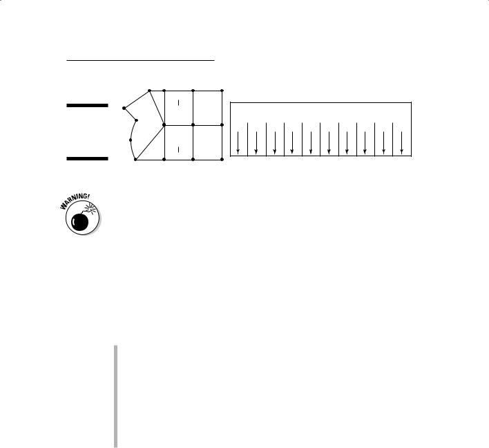
DIME recognizes the three basic components of topology (contiguity, connectivity, and area). The primary purpose of this model is to allow census data users to link the tabulated census information to census geographic units (such as streets, blocks, districts, and so on). The DIME model stores the topology by creating explicit From and To nodes that define each link for each map (as shown in Figure 5-8). Each of these links, like any topological model, includes explicit information about what’s on its left and right sides.
In Figure 5-8, the left and right sides of the link from node 21 to node 22 are census blocks 88 and 90; these blocks constitute polygons on a map showing these census divisions. DIME files also include addresses for each side of each link (left and right blocks) so that the DIME model also allows the user to easily identify and locate census divisions inside the database.
Chapter 5: Understanding the GIS Data Models |
85 |
|
Lake |
Drive |
|
|
|
Figure 5-8: |
10 |
|
The DIME |
11 |
|
|
|
|
topological |
12 |
|
data model. |
|
|
|
|
|
88
Left block
21 |
from to 22 |
|
node node |
Right block
90
89
|
From Node |
To Node |
Blocks |
Left Addr |
Right Addr |
||||||
23 |
Map Node Map Node Left Right |
Low High |
Low High |
||||||||
3 |
21 |
3 |
22 |
88 |
90 |
111 |
1999 |
102 |
189 |
||
|
|||||||||||
91
13 |
17 |
18 |
19 |
The major drawback to the DIME file is that its geography isn’t very realistic. It represents a curved street, such as Lake Drive in Figure 5-8, with a straight line. In 1980, the Census Bureau wasn’t concerned about the accuracy of such features. When others began using the DIME files for implementations other than census tabulation, the geography became more important and was added to the more advanced TIGER data structure. For example, some insurance companies use the census files to map which houses lie within zones likely to be flooded every 100 years (100-year flood zones). The improved geographic accuracy of the TIGER files is vital for accurately locating such houses.
The DIME files are still available today, although the U.S. Census Bureau has replaced them with a more advanced topological structure called Topologically Integrated Geographical Encoding and Referencing (TIGER). Advantages of TIGER files over DIME files include:
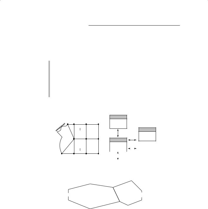
Easy retrieval: The TIGER model directly addresses points, lines, and polygons, so you can more easily retrieve a census block by retrieving the block number, rather than having to find the links first and use their topological information for retrieval. Figure 5-9 illustrates how the TIGER data model is structured.
Improved geography: Although Lake Drive is represented as a straight line in DIME files (as shown in Figure 5-8), TIGER files show the actual shape of Lake Drive (see Figure 5-9). This feature makes TIGER files much more compatible with non-census-related research and other data files that are more geographically accurate.
TIGER files are readily available both from the U.S. Bureau of the Census and third-party vendors who often repackage the files. TIGER files are compatible with a vast array of other data types, possess lots of data already in this format, and constitute an elegant implementation of the topological data model, so they’re likely to be around for a while.
Understanding the ESRI coverage approach
One of the early successful topological data models, the coverage model, developed into one of the most successful commercial GIS products of its time — the ArcInfo that ESRI uses. Each map layer is a single unit composed
86 |
Part II: Geography Goes Digital |
of geographic features associated with a common theme. Each theme covers the study area’s geographic extent, and a series of these themes represents a more comprehensive view of the content of the study area.
In a coverage, here’s how the features are stored:
Entities: Primary features such as points, arcs (the word ESRI uses for lines), and polygons
Complementary information: Secondary features such as
•Tics: Points that show the input device where the map coordinates are
•Links: Computer code that ties the graphics to the descriptions
•Annotations: The text of the descriptive information
The attribute information itself is stored in a separate set of database files.
One Cell
ke |
Drive |
|
|
La |
|
88 89
Left block
21 |
from to 22 |
23 |
|
node node |
|
Zero Cells
Nodes 18, 19...
Links
Two Cells
Blocks 85, 86, 87, 88, 89
Zip codes ...
|
|
|
|
|
|
|
Right |
|
|
|
|
|
|
|
|
|
|
|
|
|
|
|
|
|
|
|
|
|
|
|
|
|
|
|||
|
|
|
|
|
|
|
block |
|
|
|
|
|
|
|
|
|
|
|
|
|
|
|
|
|
|
|
|
|
|
|
|
|
|
|||
|
|
|
|
|
|
|
|
91 |
|
|
|
|
|
|
|
|
|
|
|
|
|
|
|
|
|
x, y |
x, y, x, y, x, y ... |
|||||||||
|
Zero Cell |
|
|
|
|
90 |
|
|
|
|
|
|
|
|
|
|
|
|
|
|
|
|
|
|
||||||||||||
|
|
|
|
|
|
|
|
|
|
|
|
|
|
|
|
|
|
|
|
|
|
|
|
|
|
|
|
|
||||||||
|
|
|
|
|
|
|
|
|
|
|
|
|
|
|
|
|
|
|
|
|
|
|
|
|
||||||||||||
|
13 |
17 |
|
|
|
|
18 |
19 |
|
|
|
|
|
|
|
|
|
|
|
|
|
|
|
|
|
|
|
|
|
|
|
|||||
|
|
|
|
|
|
|
|
|
|
|
|
|
|
|
|
|
|
|
|
|
|
|
|
|
|
|
|
|
|
|
|
|
|
|
|
|
|
|
|
|
|
|
|
|
|
|
|
|
|
|
|
|
|
|
One Cells |
|
|
|
|
|
|
|
|
|
|
|
|
|
|||||
|
|
|
|
|
|
|
|
|
|
|
|
|
|
|
|
|
|
Tract boundary, |
|
|
|
|
|
|
|
|
|
|
|
|
||||||
|
|
|
|
|
|
|
|
|
|
|
|
|
|
|
|
|
|
railway #1, ... |
|
|
|
|
|
|
|
|
|
|
|
|
|
|||||
|
|
|
|
|
|
|
|
|
|
|
|
|
|
|
|
|
|
|
|
|
|
|
|
|
|
|
|
|
|
|
|
|
|
|
|
|
|
|
|
|
|
|
|
|
|
|
|
5 |
|
|
|
|
|
|
|
|
|
|
|
|
3 |
|
|
|
|
|
|
|
|
|
|
||
|
|
|
|
|
|
|
|
|
|
|
|
|
|
|
|
|
|
|
|
|
|
|
|
|
|
|
|
|
|
|
|
|
|
|
|
|
|
|
|
|
|
|
|
|
|
|
|
|
|
|
|
|
|
|
|
|
3 |
|
|
|
|
|
|
|
|
|
|
|
|
|
|
|
|
|
|
|
|
|
|
|
|
|
|
|
|
|
|
7 |
|
|
|
4 |
|
|
|
|
|
|
|
|
|
2 |
|
|
|
|
|
|
|
|
|
|
|
6 |
|
|
|
8 |
|
|
|
|
|
|
|
|
|
2 |
|
|
|
|
|
2 |
|
||||||||||||
|
|
|
|
|
|
|
|
|
|
|
|
|
|
|
|
|
|
|
|
|
|
|
|
|
||||||||||||
|
|
|
|
|
|
|
|
|
|
|
|
|
|
|
|
|
|
|
|
|
|
|
|
|||||||||||||
|
|
|
|
|
|
|
|
|
|
|
|
|
|
|
|
|
|
|
|
|
|
|
|
|
|
|
|
|
||||||||
|
|
|
|
|
|
|
|
|
|
|
|
|
|
|
|
|
|
|
|
|
|
|
|
|
|
|
|
|||||||||
|
|
|
|
|
|
|
|
|
|
|
|
|
|
|
|
|
|
|
|
|
|
|
|
|
|
|
|
|||||||||
|
|
|
|
|
|
|
|
|
|
|
|
|
|
|
|
|
|
|
|
|
|
|
|
|
|
|
|
|
|
|
|
|
|
|||
|
|
|
|
|
|
|
|
|
|
|
|
|
|
|
|
|
|
|
|
|
|
|
|
|
|
|
|
1 |
|
|
|
|
||||
|
|
|
|
9 |
|
|
|
|
|
|
|
1 |
|
|
|
|
|
|
|
|
|
|
|
|
|
|
|
|
|
|||||||
|
|
|
|
|
|
|
|
|
|
|
|
|
|
|
|
|
|
|
|
|
|
|
|
|
|
|
|
|
|
|
|
|||||
|
|
|
|
|
|
|
|
|
|
|
|
|
|
|
|
|
|
|
|
|
|
|
|
|
|
|||||||||||
|
|
|
|
|
|
|
|
|
|
|
|
|
|
|
|
|
|
|
|
|
|
|
|
|
|
|
|
|
|
|
|
|
|
|
|
|
|
|
|
7 |
|
|
|
|
|
|
|
|
|
|
|
|
|
|
|
|
|
|
|
|
|
|
|
|
|
|
|
|
1 |
|
|
||
|
|
|
|
|
|
|
|
|
|
|
|
|
|
|
|
|
9 |
|
|
|
|
|
|
|
|
|
6 |
|
|
|
|
|
||||
|
|
|
|
|
|
|
|
|
|
|
|
|
|
|
|
|
|
|
5 |
|
|
|
|
|
|
|
|
|
||||||||
|
|
|
|
|
10 |
|
|
|
|
|
|
|
|
|
|
|
|
|
|
|
|
|
|
|
|
|
||||||||||
|
|
|
|
|
|
|
8 |
|
|
|
11 |
|
|
|
|
10 |
|
|
|
|
|
|
|
|
|
|||||||||||
|
|
|
|
|
|
|
|
|
|
|
|
|
|
|
|
|
|
|
|
|
|
|
|
|
|
|||||||||||
|
|
|
|
|
|
|
|
|
|
|
|
|
|
|
|
|
|
|
|
|
|
|
|
|
|
|||||||||||
|
|
|
|
|
|
|
|
|
|
|
|
|
|
|
|
|
|
|
|
|
|
|
|
|
|
|
|
|
|
|
|
|
|
|||
|
|
|
|
|
|
|
|
|
|
|
|
|
|
|
|
|
|
|
|
|
|
|
|
|
|
|
|
|
|
|
|
|
|
|||
|
|
|
|
|
|
|
|
|
|
|
|
|
|
|
|
|
|
|
|
|
|
|
|
|
|
|
|
|
|
|
|
|
|
|
|
|
|
|
|
|
|
|
|
|
|
|
|
|
|
|
|
|
|
|
|
|
|
|
|
|
|
|
|
|
|
|
|
|
|
|
|
||
|
|
Polygons |
|
Chain |
|
|
|
|
|
|
|
|
|
Chains |
|
|
|
|
|
|
|
|
||||||||||||||
|
|
|
|
list |
|
|
|
|
|
|
|
|
|
|
|
|
|
|
|
|
|
|||||||||||||||
|
|
|
|
|
|
|
|
|
|
|
|
|
|
|
|
|
|
|
|
|
|
|
|
|
|
|
|
|
|
|
|
|
|
|||
|
|
Polygon Polygon |
Chain |
Chain |
|
Chain points |
Chain |
From |
|
|
To |
|
Left |
|
|
Right |
|
|||||||||||||||||||
|
||||||||||||||||||||||||||||||||||||
Figure 5-9: |
|
name |
|
pointer |
|
list |
name |
|
(X, Y strings) |
length |
node |
|
node |
polygon polygon |
|
|||||||||||||||||||||
|
1 |
|
– |
|
4 |
|
|
4 |
|
x, y, x, y |
– |
|
4 |
|
|
9 |
|
|
2 |
|
1 |
|
||||||||||||||
The TIGER |
|
2 |
|
– |
|
5 |
|
|
5 |
|
|
– |
– |
|
|
– |
|
|
– |
|
|
– |
|
|
– |
|
||||||||||
topological |
|
– |
|
– |
|
6 |
|
|
6 |
|
|
– |
– |
|
|
– |
|
|
– |
|
|
– |
|
|
– |
|
||||||||||
data model. |
|
– |
|
– |
|
|
– |
– |
|
|
– |
– |
|
|
– |
|
|
– |
|
|
– |
|
|
– |
|
|||||||||||
|
|
– |
|
– |
|
|
– |
– |
|
|
– |
– |
|
|
– |
|
|
– |
|
|
– |
|
|
– |
|
|||||||||||

Chapter 5: Understanding the GIS Data Models |
87 |
The coverage model supports the three major properties of topology: contiguity, connectivity, and area definition. The coverage model has been around for over two and a half decades, but most GIS software vendors still support it because of the large number of GIS users whose data were (or still are, in some cases) stored as coverages.
Working with object-oriented representations
Advances in computer languages and their associated data structures — the development of object-oriented programming (OOP) — brought about a useful adoption for GIS data models. OOP focuses on objects where an object is a set of computer code that can be copied from place to place in a computer program. In GIS, an object represents a type of geographic feature that you can move around and whose properties follow it (are inherited) no matter where you place it. Incorporating OOP languages resulted in wholesale rewriting of some GIS software and development of new software based entirely on this model.
Much of the power of OOP data models results from the objects’ shared properties, or the characteristics they have in common with other objects in their group. (I describe the sharing of properties briefly in the sidebar, “Sharing the property,” and talk more about object structure in Chapter 6.) Because of shared properties, an object always knows what it can and can’t do, and what it can and can’t support. So, you don’t have to worry about any surprises when you retrieve information from an object-oriented GIS. If you’re looking for information on a land parcel, you won’t pull data related to oceans because the ocean objects don’t share the properties of (and, so, aren’t grouped with) land parcel objects.
You can find several implementations of the object-oriented model available, including the ESRI Map Objects product and the GE Smallworld GIS product.
Taking on advanced geographic representations
Perhaps the most robust and advanced of the object-oriented models is the ESRI new geodatabase model. The geodatabase (not to be confused with a collection of geocoded data inside a GIS software package that’s sometimes referred to as a geodatabase) allows you to store a wide variety of data types (including raster, vector, CAD, and others) in the same system. Here’s a quick list of the types of data this model can incorporate:
Attribute tables from typical RDBMS (see Chapter 6).
Geographic features that you might find in land-use maps.
Satellite and other digital imagery such as the files you might get from the LANDSAT satellite.
Surface models you could obtain from the USGS Digital Elevation Models (DEMs).
Survey data from scientific vegetation samples, or telephone surveys, for example.

88 |
Part II: Geography Goes Digital |
|
|
|
|
||
|
|
||
|
|
||
|
Sharing the property |
||
|
In object-oriented models, geographic features |
larger group of polygons called parcels. The par- |
|
|
are stored as objects. There’s debate about |
cels in this group share a set of conditions that |
|
|
exactly what an object is, but in GIS, an individual |
differ only in the specifics. For example, all the |
|
|
object (with its local properties) also represents |
parcel objects have a type of land use, an owner, |
|
|
a group of objects that has a set of more global |
and zoning restrictions. So, the general proper- |
|
|
properties. By being part of the group, the object |
ties outlined for a parcel object (meaning that it |
|
|
shares those global properties. So, for example, |
has a land-use type, an owner name, and a set of |
|
|
a land parcel object has unique identifiers — |
zoning restrictions) are inherited by every other |
|
|
owners, value, size, shape, and so on — but |
parcel. |
|
|
it still possess a set of properties shared by a |
|
|
|
|
|
|
|
|
|
|
The geodatabase model, like the non-object-oriented coverage model, has tables of data that include objects (rows in the database table) and features (objects that have explicitly defined geometry). It’s a completely topological model, like its predecessors. What makes the geodatabase so powerful is that each of these objects can contain a wide array of rules and logic, which makes the objects more like real geographic objects. For example, if you have a geodatabase of electrical infrastructure, certain lines that represent a type of wiring don’t connect to non-compatible types of wiring because the database explicitly stores properties that prohibit such a dangerous connection. Or, if you have a road-network geodatabase, the rules might prohibit you from connecting a one-way street going east to another one-way street going west.
Although the geodatabase is new and quite different from its non-object-oriented cousins, it has a lot of tools that you can use to migrate your data to the geodatabase format. While GIS analysis becomes both more sophisticated and more realistic, the geodatabase and other object-oriented models like it will increase their capacity to represent rules and conditions that characterize real-world geographic features.
ESRI has made many industry-specific geodatabase models that contain complete logic available for use, so you don’t need to build them from scratch. If you’re looking for a GIS for a specific application, check to see whether ESRI has the model you need before reinventing the wheel.
Chapter 5: Understanding the GIS Data Models |
89 |
Dealing with Surfaces
Surfaces of all kinds are very common in GIS, but because of their threedimensional nature, they place additional demands on the computer programmer who wants to represent them. Beyond having to represent the X and Y coordinate, and the associated attributes, you also have to worry
about how to effectively include the third dimension in such a way that the software can perform all the basic operations on surfaces that the other data types allow, such as storing, retrieving, editing, analyzing, comparing, and outputting.
Storing surface data in a raster model
The general raster model provides the easiest method of storing surface data. Each grid cell represents not just an area on the surface of the Earth, but also a single elevation value. So, a grid cell in column X and row Y would store a single value Z that represents the elevation for the entire grid cell (as shown in Figure 5-10).
This model does limit the accuracy of your elevation values, just like the raster model itself limits the locational accuracy and spatial representation of the actual geography (see “Making a quality difference with resolution,” earlier in the chapter). On the plus side, the model does allow for some very nice surface modeling with low computational overhead (far fewer calculations), and you can easily convert it to other forms of surface representation.
Figure 5-10:
A raster representation of surface data.

90 |
Part II: Geography Goes Digital |
The most common form of raster surface model is called the Digital Elevation Model (DEM), which was developed by the United States Geological Survey (USGS) to store and eventually process topographical surface data. DEMs are a series of regularly placed X and Y coordinate locations that also contain Z values, which depict the topographic elevations at those locations.
DEMs come in a number of different sizes, based on the maps from which they were derived. USGS DEMs come in 7.5-minute (meaning 7.5 minutes of latitude by 7.5 minutes of longitude each), 15-minute, 30-minute, and 1-degree versions. The 7.5-minute series provides the most elevational detail. When you move from 7.5 minutes to 1 degree, you lose both horizontal and vertical accuracy.
You can get the DEM directly from the USGS, and it’s also available from other vendors as a value-added product. Most modern GIS packages support the DEM data model, which allows you to convert the data in the model from its original form as a matrix of X, Y, and Z values to raster grid-cell structure, contour lines, and even vector topographic data models.
Representing surfaces in a vector model
Trying to represent surfaces in vector models is a bit more complex than in raster models, but the basic idea for this model has been around since the early 1960s. Based on the idea that many parts of a surface are relatively flat, the programmers constructed a model that looks much like how three-dimen- sional computer characters (avatars) are constructed.
The primary vector model that represents surfaces in the computer is called the Triangulated Irregular Network (TIN), shown in Figure 5-11. The words in the TIN’s name really explain what it does:
Triangulated: The locations (X, Y, and Z coordinates) are created through a process of triangulation (a method of surveying based on the trigonometric properties of a triangle) and are represented as a set of non-overlapping triangles.
Irregular: These triangles are irregular in shape because each represents a flat portion (facet) of the overall surface.
Network: The triangles are joined together edge-to-edge to create a surface.
Each triangle is like the facet of a crystal. In this case, however, the crystal is a portion of the topographic surface. The three vertices (points of the triangle) of each facet (non-overlapping triangle) each have X and Y coordinates, and each has a unique elevation value. The slope (angle from horizontal) and aspect (direction) are uniform and constant for each individual triangle.