

GIS For Dummies
.pdfChapter 4: Creating a Conceptual Model |
71 |
Weighing the benefits:
Raster versus vector
You may wonder how you should decide whether you need raster or vector data (described in the preceding sections) — or both — in your GIS operation. The raster-versus-vector debate is far less important today than it was in the past. Most modern GIS software has both raster and vector data components, or it can convert from one format to another. You need to determine the most important functionality, accuracy, and storage issues for the work you want to do when you decide on GIS software.
So, to help you make your decision, here’s my nutshell look at the differences between raster and vector data models:
Raster data takes up more computer space than vector data. Space may not be a serious issue unless you know that you have limited computer storage and can’t get any more. Raster data require that each grid cell have an associated value, but as few as three sets of X and Y coordinate pairs can represent large areas in vector data.
Raster is faster (computationally) than vector. With computer speed rapidly increasing, this speed difference might not seem a huge issue, but the spatial datasets that GIS use are increasing in size at an even faster pace. So, if you have GIS applications that involve many datasets, you may want to use the computationally faster raster data.
Raster is compatible with much scanned and remotely sensed data.
Many raster datasets, usually in the form of scanned images (aerial photography) or satellite images, are quite useful in GIS analysis. Because they are similar data structures, you don’t need to do a lot of data conversion to add them to your GIS. Determine what datasets your application needs and keep those datasets in mind when you choose your data structure.
Raster is less spatially accurate than vector. A lot of people believe that vector data gives an accurate representation of locations in geographic space, but that belief isn’t entirely true. Computers can’t represent geographic space exactly because each computer’s internal computational accuracies vary. Computers often truncate or round up numbers, have single or double precision (the number of points beyond the decimal point that they round to), and manipulate numbers by using algorithms that do strange things (other than rounding) to the numbers. Even so, the spatial accuracy of vector is much better than that of raster, where the resolution (spatial dimension) of the grid cells determines accuracy. The smaller the grid-cell size, the more accurately it represents geographic space.
72 |
Part II: Geography Goes Digital |
Raster data give you more options to work with surfaces than vector data. Because each grid cell has a unique surface value, any measurement made over the entire surface can reflect these unique values, whereas with vector data (the TIN model), the computer assumes that large parts of the surface have the same value (the triangular plane’s slope).
Raster generally provides visually less desirable output (especially with its coarser resolution) than vector. Some map readers dislike maps represented as grid cells because the lines and edges do not appear smooth like they would in paper maps.
Raster is more powerful for modeling than vector. One other factor, and an important one for the modeler, is that you can use raster data much more efficiently as data for modeling because it gives you far more options. In Chapter 18, you can examine the detail of the Map Algebra modeling language that was originally developed for the raster data model. You can use the language to perform complex processes, called cartographic modeling, with more than just raster data, but the language has far more options with raster data. The raster data model has nearly limitless and extremely powerful (complex and accurate) modeling capabilities.
Raster is more compatible with printer output technology and less compatible with plotter output technology than vector. (A plotter is a type of printer that draws lines rather than printing a series of dots.) Raster and vector models in the GIS software must communicate with hardware for input and output. Each input and output device also has its own coordinate system and its own data structure (whether raster or vector).
You can convert the data captured by most input devices — whether vector (as in the case of digitizers) or raster (as in the case of scanners) — from one to the other data model without much loss of accuracy. On the other hand, plotters tend to be vector based, and printers tend to be raster based. The compatibility of your GIS data model with that of your input and output devices becomes a factor in determining the quality of your output.
Check out Chapter 22 for guidance on selecting a GIS vendor.

Chapter 5
Understanding the
GIS Data Models
In This Chapter
Finding your way around a raster representation
Exploring vector models
Entering surfaces into the computer
When you read a map, you must be able to visualize what the real world represented by the map looks like. As a GIS analyst, you need
an understanding that goes beyond looks because you use this symbolic information to analyze and combine data, and more importantly, make decisions about the space that the map represents. In some cases, you lose the graphical elegance of a paper map in the computer version because the computer emphasizes computational effectiveness over good looks.
In this chapter, I help you understand how the data models that the software uses work so that you understand both the limitations and the power of a GIS.
Examining Raster Models and Structure
A checkerboard represents a unit of space divided into squares upon which the checkers rest. Likewise, raster GIS grids (the checkerboard) are broken up into grid cells (the squares) upon which geographic features (plants, animals, houses, towns, rivers, and so on) rest. On a checkerboard, the checkers are like occupants of the geographic space — you can move them around in different places. But the checkers have to stay on the dark-colored squares and move between them diagonally. In other words, the checkerboard restricts where you can place features (checkers) and where you can move them. Similarly, geographic space has limitations about what can and can’t occur.
74 |
Part II: Geography Goes Digital |
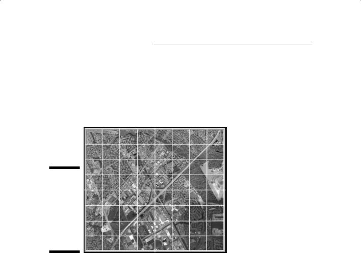
In the real world, the nature of physical features imposes rules that control or limit what things can or should occupy different spaces. For example, you can’t build houses in the middle of a river, and you can’t sail boats on dry land. But the real world doesn’t consist of alternating squares of water and land; the makeup of the Earth is much more complex than that. Figure 5-1 shows a grid overlaid on a map that depicts a more typical distribution of land and water features.
Figure 5-1:
A grid overlay shows how each square represents
aportion of real
geographic space.
Representing dimension when everything is square
If geographic space were exactly like a checkerboard, it would be composed of square areas, each containing a given category of Earth surface data. But real geographic space contains more than area (or polygon) features. Real geography has point, line, and surface (or volume) features that must also show up in the grid structure.
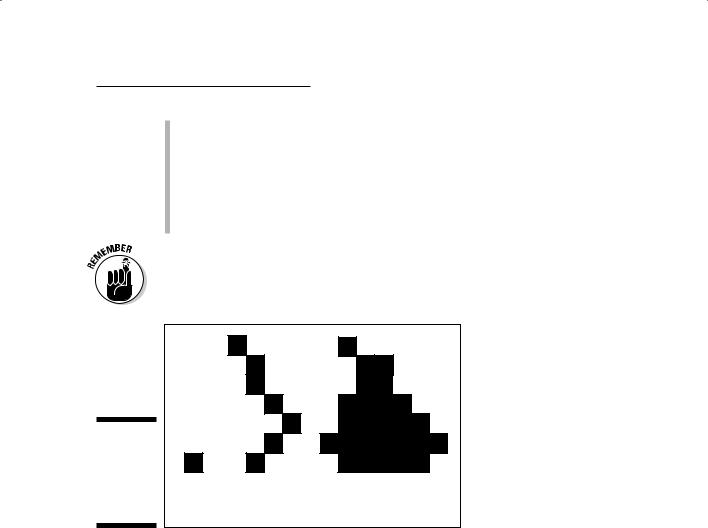
Surfaces require that the grid system represent a third dimension (and a bit more complexity); I discuss how the computer represents surfaces in the section “Dealing with Surfaces,” later in this chapter. In this list, I show you how to represent features that have two dimensions or less by using grid cells (see Figure 5-2):
Chapter 5: Understanding the GIS Data Models |
75 |
Points: Even though points are considered zero-dimensional objects that don’t take up any space, they’re still included in the raster representation as a single grid cell.
Lines: Features represented as lines (one-dimensional objects) are composed of a string of grid cells.
Areas: By definition, areas are two-dimensional objects, and they show up as groups of grid cells.
In raster GIS, points are single grid cells, lines are strings of grid cells, and areas are groups of grid cells. See Chapter 4 for a more complete discussion of how grids represent geographic features.
Figure 5-2: |
|
|
|
Point, line, |
|
|
|
and area |
|
|
|
features in |
|
|
|
the raster |
|
|
|
data model. |
Point |
Line |
Area |
Making a quality difference with resolution
At first glance, representing zeroand one-dimensional objects with twodimensional grid cells doesn’t seem to make much sense. But the raster model is just a way of representing geographic space and its features to help you store related information in the computer.
The spatial accuracy does suffer with these grid cells, especially for points and lines. This data model compromises both the exact location and the amount of space occupied. But this limitation in spatial accuracy is the necessary trade-off with the power of the raster data model for performing highquality geographic modeling. Given this trade-off, you have one good way to
76 |
Part II: Geography Goes Digital |
improve the spatial quality of grid cells — make them smaller. Like with a high-definition television, the smaller the dots, the higher the resolution, and the more accurate the representation. In raster GIS, this concept is called the grid cell resolution.
In raster GIS, the smaller the grid cell size, the finer its resolution, and the more accurately those cells represent the location and spatial extent of the geographic features.
Finding objects by coordinates
The raster coordinate system is a set of sequential numbers that identify the column (X) and row (Y) locations of each grid cell. The sequence usually starts with the upper-left corner of the grid and moves from left to right across the columns and from top to bottom down the rows (see Figure 5-3). This X and Y coordinate system is pretty standard, but it doesn’t preclude starting, for example, on the bottom left and counting up and to the right. In any case, all grid coordinate systems do basically the same thing — they locate the positions of grid cells based on columns and rows.
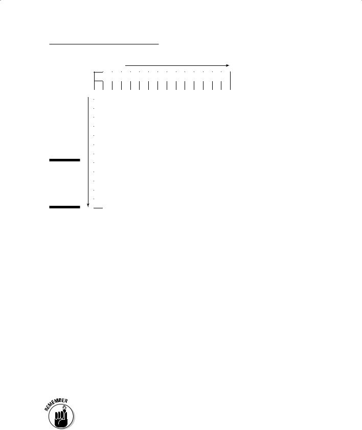
Because the grid-cell resolution represents real geographic space, any movement from one cell to another constitutes a symbolic traverse of both distance and direction in geographic space. For example, if you set your grid-cell resolution at 100 meters, each grid cell is 100 meters on a side and has an area that you can calculate as follows:
100 × 100 = 10,000 square meters
So, if you start at the upper-left corner of a map represented this way and move 15 grid cells to the right, you’re in grid column 15 and grid row 1. It also means that you traveled 15 times the length of each grid cell (1,500 meters). And you can link this distance and direction directly to the geographic grid (latitude and longitude), which means that you traveled 1,500 meters east from your starting point. Likewise, if you move down a column, you can envision that you’re moving south.
This system allows you to find virtually any object by its column and row coordinates. And, because these column and row coordinates are linked to the geographic grid, you can easily relate the grid cells to specific positions on the Earth. More important for the GIS modeler, you can layer grids and relate the corresponding grid cells to each other. Using layered grids for modeling requires that
All the grids represent the same portion of the Earth.
Grids are co-registered (meaning they lie directly on top of one another).
Each grid cell is the same size in every map layer.
Chapter 5: Understanding the GIS Data Models |
77 |
Columns


 Rows
Rows
Figure 5-3:
A typical raster grid coordinate system.
The really cool thing about having these grid cells co-registered is that you can compare lots of different features that occur in the same geographic location but appear on different map layers. For example, you can compare the location of a building (on the land-use layer) with its soil (on the soil-type layer) and the existence of a hazardous chemical found in that soil (on the soil-chemistry layer), all because the locations of each set of grid cells are right on top of each other in the various map layers.
Finding grid cells by category
Each grid cell in a raster GIS has a unique set of X and Y coordinates, and each group of cells has different properties. Unlike the squares on a checkerboard, grid cells come in as many types as you have categories to include in your map.
Because the raster data model structures grid cells into a coordinate system, you can find any grid cell you want by simply determining its column and row location (X and Y coordinates). Because you can also assign a category (a particular type, class, or even value) to each grid cell, line of grid cells, or group of grid cells, you give yourself another way of finding them. That is, after you make the assignments, you can search the grid by categories, as well as by coordinates.
Raster GIS gives you the power to search the grid in two ways. You can search by coordinates to examine what the grid cell represents, or you can search by grid-cell quality to find out where grid cells with that quality are located.
78 |
Part II: Geography Goes Digital |
Working with map layers
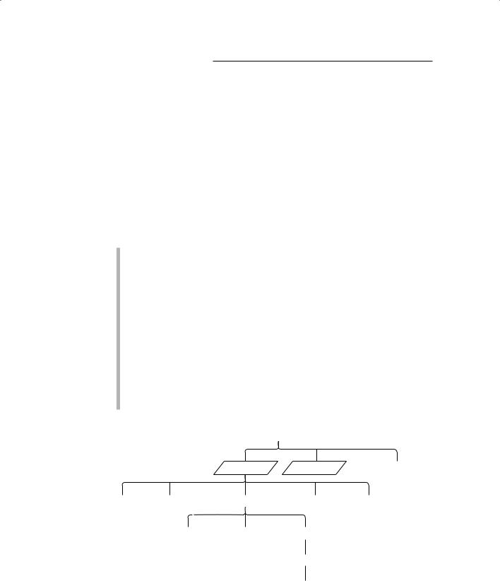
When raster GIS was first developing, software programmers made different attempts to create a storage and recordkeeping system that would allow the user to input, store, retrieve, manipulate, compare, and output grids. Perhaps the most successful, called the Map Analysis Package (MAP), presents maps as a series of layers, each with a different name. First, you find the map layer that you need. You retrieve map layers by searching for the map name (the theme). Each map has a set of categories, each category with a unique number value that can be retrieved individually. These categories also have labels associated with them for display. Figure 5-4 illustrates the MAP raster data model.
The MAP data model breaks down into these components (from the most general to most specific):
Theme: The major unit of retrieval. In Figure 5-4, the map themes are called GRID LAYER 1, GRID LAYER 2, and so on.
Category: After you retrieve a map, you’re free to search the multiple categories within the map’s theme. This data model represents each of these descriptive attributes with a unique numerical value (for example, Category1 in Figure 5-4). Modern raster GIS software allows you to search these categories by name.
Value: Numbers that represent the categories. You use those numbers to do your analysis. In other words, the computer actually retrieves, compares, and analyzes the numbers themselves rather than the categories they represent. A GIS locates the category values associated with sets of points (grid cells) by their X and Y coordinates. Having category values associated with grid-cell locations is essential for doing overlays (Chapter 16) and for using the modeling language called map algebra, which I describe in Chapter 17.
|
|
|
|
Map file |
|
|
|
|
GRID LAYER 1 |
GRID LAYER 2 |
GRID LAYER n |
|
Title |
Grid cell resolution |
Category 1 |
Category 2 |
Category n |
|
|||||
Figure 5-4: |
|
|
|
|
|
The Map |
label |
display symbol |
attribute value |
|
|
Analysis |
|
||||
Package |
|
|
|
|
|
(MAP) |
|
|
set of points |
|
|
raster data |
|
|
|
|
|
model. |
|
|
X,Y coordinates |
|
|
|
|
|
|
|
|
|
|
|
|
|
|

Chapter 5: Understanding the GIS Data Models |
79 |
Linking objects and descriptions
The Map Analysis Package (MAP) data model makes it easy to find individual categories in a single thematic grid. Its limitation is that, as originally designed, the MAP data model represents each category only once per layer. The solution is simplicity itself. For each map, you add not just categories, but also a database of categories by linking the map to a database management system. The database management system can store multiple values for each category. So, now you can have a map of land use that includes a category called housing, and that category can have many different subcategories. Raster software such as the Spatial Analyst that the Environmental Systems Research Institute (ESRI) uses currently implements this model.
Extending the raster data model by including a database management system gives you a lot more flexibility. But you need to make sure that you know where to look for the categories and that you give them names you can remember. Always use meaningful and memorable names for categories, ID-codes (codes you use for categories), and maps, if at all possible.
Exploring Vector Representation
To think about maps inside the computer in a graphically familiar way (think paper map), envision each point as a point with its own X and Y coordinates, each line with an ordered set of these coordinate pairs, and each polygon with a string of points that close (begin and end at the same place). Conceptually, vector GIS software both stores and displays points and lines more accurately, making those points and lines nearly zeroand one-dimensional, respectively, and having polygons more closely represent their own shape. The closer together the points that make up line segments, the more accurately they represent the real lines.
Several data models allow the conversion, storage, and manipulation of map data by using the vector approach. Some of these models are simple and work very well for input and output devices, and others are more complex and allow for some serious computational power.
Simple forms of vector representation
Simple forms of vector representation focus more on the accurate graphic depiction of features and less on the subsequent analysis of geographic information. The simple forms still in use today are mostly for input and output, rather than actual GIS functionality. Modern GIS software communicates quite effectively with these feature-depicting models, which often come builtin to the GIS as graphics languages.

80 |
Part II: Geography Goes Digital |
This ability to communicate with graphics depiction models is necessary because even the most complex data modeling can’t happen if you can’t get data into the GIS software or create a map when you’re done with your analysis.
Spaghetti representation
The simplest of vector data models is the spaghetti model (see Figure 5-5), a one-to-one translation of graphics into the computer without regard for
spatial relationships. Software using the spaghetti model stores points in the computer with identifying numbers (for example, the first point is number 1, the second is number 2, and so on). Each number is linked directly to its corresponding X and Y coordinates in a separate data table. Lines are ordered strings of points (the spaghetti), each associated with a searchable point identification number. Finally, the software stores the polygons, which also have searchable IDs, as closed loops of coordinate pairs.
The spaghetti model is simple, easy to understand, and (more importantly) fast for both input and output. It doesn’t work — meaning it doesn’t store information correctly — when you try to represent features such as islands because they’re effectively a polygon within a polygon. The data model also doesn’t recognize polygons comprised of non-contiguous parts, such as island chains. These data representation limitations make this data model ineffective for modeling and analysis.
Alternative representation
One vector data model created by ESRI gives much more control than the spaghetti model. Instead of limiting storage of points, lines, and polygons to coordinate pairs, this model (called a shapefile) stores the geometry of each feature as a shape that contains the coordinates and links to the attributes. GIS software packages widely use this data model today because of its relatively low processing overhead, low storage requirements, fast drawing speeds, and its ability to handle overlaps and non-contiguous features. You can also, with relative ease, convert the shapefile model to more complex data models, which I describe in the section “Complex forms of Vector Representation,” later in this chapter.
The term shapefile is a bit misleading. A shapefile isn’t a single file. Instead, it’s three separate files that allow for the representation of 14 different types of geometric shapes (as outlined in Figure 5-6). The primary file with an .shp extension is a list of X and Y coordinates that define objects called shapes. To keep track of the shapes and search them by type, it also has an index file that has a file extension .shx. Finally, the .dbf (or database) file contains all the attributes that describe the features.
Although the shapefile is still a fairly simple data model, compared to some of the more advanced ones, it’s likely to be a GIS software mainstay data model for years to come because it’s simple and compatible with many software programs.