

GIS For Dummies
.pdfChapter 13: Working with Statistical Surfaces 201
Understanding discrete and continuous surfaces
Surfaces can be discrete or continuous. A discrete surface results from mapping Z values that occur only in certain places in space. They don’t occur at every point in the geographic space covered by the map. People, plants, animals, houses, and parked cars are all examples of features that you can map as Z values and that occur in discrete locations. Because discrete surfaces occupy separate and distinct places in space, they appear blocky rather than smooth, as illustrated in Figure 13-2.
Figure 13-2: |
|
A side |
|
view of |
|
continuous |
|
and discrete |
|
surfaces. |
|
Continuous |
Discrete |
Continuous surfaces (also depicted in Figure 13-2) include all features that occur everywhere — meaning that every part of the surface has a measurable value. Temperature, barometric pressure, and elevation all occur everywhere. Because they occur everywhere — at all points of the mapped area — an infinite number of them exist.
When you work with continuous surfaces, you work with an infinite number of data points. If you tried to include all this data in one GIS database, you’d need that database to have infinite storage capability — which just isn’t possible.
So, you sample from the total and hope that the sample represents the total population with an acceptable degree of accuracy.
The section “Sampling statistical surfaces,” later in this chapter, covers the specifics of sampling procedures.
Exploring rugged and smooth surfaces
Surfaces can change slowly or abruptly, and you can classify these surfaces as rugged (as in rugged terrain) or smooth. The ruggedness or smoothness of a surface hints at characteristics of that surface. You can travel over gradual changes in topography much more easily than you can travel across abrupt changes, which signify rugged terrain; gradual changes in barometric
202 Part IV: Analyzing Geographic Patterns
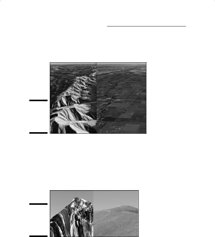
pressure produce less variable weather patterns than abrupt changes; and gradual changes in soil nutrient levels result in less variable crop yields than abrupt shifts in soil nutrients. Figure 13-3 shows an example of rugged versus smooth terrain.
Figure 13-3:
Rugged (left) versus smooth (right) terrain.
Climbing steep surfaces
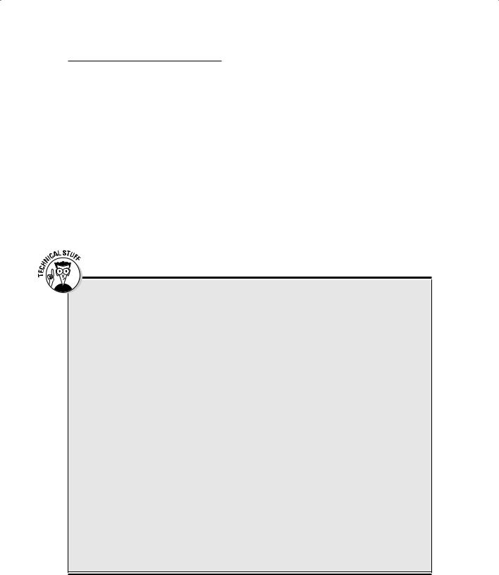
Like ruggedness, the steepness (change in Z value over distance) of a surface has an impact on surface characteristics. Steep slopes require more fuel consumption for uphill travel, steep changes in depth of an ore body change the amount of surface material that you must remove to access the ore, and steep changes in barometric pressure result in high winds. Figure 13-4 shows steep versus gentle topographic slopes.
Figure 13-4:
Steep (left) versus gentle (right) topographic slopes.
Chapter 13: Working with Statistical Surfaces 203
Determining slope and orientation
Slope is basically the measure of steepness for any statistical surface. It is essentially a comparison of how rapidly the Z values change as you move across the X and Y (horizontal) part of the surface. Any slope is positioned at a particular angle to the horizontal (the gradient), and you can measure that angle, figure out the nature or extent of the forces that formed it, and see how it affects other surface factors by its nature.
The concepts of slope and gradient apply most often to topographic surfaces, but not exclusively. For example, the slope of a population distribution indicates how quickly population changes from one place to another. Barometricpressure slope often determines wind speeds. Rapid changes (slopes) in crime values typically mean that a local area has a location that experiences high levels of crime (a hot spot). You could come up with a quite large list of possible slopes and their explanations and/or consequences.
The math behind slope and orientation
Slope and orientation are complementary functions, and you generally calculate them simultaneously. Here’s a brief look at how you do the math to determine slope and orientation:
Slope: The amount of slope is based on the change in Z value over the change in horizontal distance. This ratio is sometimes called rise over run. In fact, you calculate slope by dividing rise by run. If you’re using elevation, you might detect that over a distance of 8 miles, the elevation has increased or decreased (depending on your direction) by 40 feet. The equation (rise/run) would be 40 feet divided by 8 miles. If you divide 40 by 8, you get a slope or gradient of 5 feet per mile (5 ft/mi).
You can also calculate slope by percent slope. To do this calculation, you need to have the numerator and the denominator in the same units. So, for example, a change in elevation of 200 feet (rise) for every 1,000 feet of distance (run) gives you 2/10 or 0.2. If you multiply 0.2 by 100, you get a 20-percent
slope. If you want to measure your slope in degrees, apply fancy inverse trigonometric functions. But most GIS applications usually rely on the two basic methods I outline. If you want to see all three of these methods side by side, you might visit
http://geology.isu.edu/geostac/ Field_Exercise/topomaps/ slope_calc.htm
Orientation: You usually hear orientation compared to compass direction. Good compasses are normally calibrated to 360 degrees, where 0 and 360 are the north direction. Not all GIS software follows this method of determining direction (for example, 0 might be east rather than north), nor does it all calibrate in 360-degree segments. Some GIS start numbering clockwise from east (0), and some reduce the number of segments from 360 to a smaller set of numbers to save computer space and speed up calculations.

204 Part IV: Analyzing Geographic Patterns
The direction in which a surface changes (orientation) is also very telling. For population data, it tells you where population is increasing and where it’s decreasing. Barometric surface orientation tells you the direction of the wind. The orientation of depth to ore body data gives mining engineers an idea of where the ore body is large and where it’s small. You can find many possible applications of surface-change directions.
Working with Surface Data
The idea of a geographic surface means that categories of geographic features have Z values (for a third dimension) that occur in different places. Z values are recorded data, called statistics. Statistical surfaces have three properties:
They contain Z values distributed across geographic space. Because you know that your data are distributed throughout the surface, you can predict values in places where you don’t have sample data.
They’re measured and recorded at interval or ratio scales. Because your data are interval or ratio scale numbers, you have really precise statistical numbers to analyze, rather than just names or “big, medium, and small” ordinal measurements.
You can assume that they’re distributed continuously. A continuous surface means that data points exist everywhere and that you can predict them. But if you have a discrete dataset, such as population by county across the lower 48 states, you can still do some of this.
These three factors give you serious power to manipulate the statistics to predict missing values and group data based on your needs. The following sections show you how to sample and analyze the statistical surface. And, like always, rules are made to be ignored. You get the scoop on which rules you can ignore, and when and how to ignore them, in the section “Ignoring the rules,” later in this chapter.
Collecting surface data for entire areas
Topographic surface data are usually collected at point locations with survey instruments and GPS units. Sometimes, however, data are collected for a whole area all at the same time. If you want to show a map of population across the lower 48 states of the United States, you can’t possibly know where each person is standing at any given time, so you collect data by some political subdivisions, such as counties. So, each county gets only one number.

Chapter 13: Working with Statistical Surfaces 205
You can map both of these datasets (topography or population by county). You can even make the discrete data collected by county look like data collected at point locations. I explain the difference in the section “Understanding Discrete and Continuous Surfaces,” earlier in this chapter.
Sampling statistical surfaces
Continuous statistical surfaces require sampling because the data occur everywhere. You can sample a surface by following these steps:
1.Examine what the surface looks like.
Take a look at the highs and lows of your surface, and get a feel for its overall structure.
2.Locate where the surface is smooth and where it is rugged.
Smooth surfaces have little change in Z value over distance while rugged surfaces change rapidly over distance.
3.Define a sampling strategy (how many samples to take and where to take them) based on your understanding of the surface change.
For example, setting a strategy based on surface change may mean that you take more samples for rugged surfaces.
Sampling surface data requires you to know something about the surface. A general guide is that the more rugged the surface, the more samples you need to take because a rugged surface has more changes in Z value than a smooth surface. Smooth surfaces have less information (defined as change in Z value over horizontal surface) than rugged ones. When you want to rep-
resent a smooth surface, you don’t need to take as many samples to capture the information as with a rugged surface.
Taking a lot of samples of a surface doesn’t necessarily increase the quality of your map. This fact is called the point of diminishing returns. Computer programs don’t actually need all the data to perform their interpolations, and you can reach a point of diminishing returns in which you gain little or no benefit by adding more sample points. The software might not even use all the additional points you provide. Not to mention, taking more samples requires more effort, which typically costs money. All that overhead, and you may not even improve the quality of your map!
Sampling statistical surfaces requires more than just knowledge of where the information content is the highest (that is, where there are rapid changes in Z value with distance), although that knowledge is extremely important.

206 Part IV: Analyzing Geographic Patterns
To define statistical surfaces, you don’t need to provide continuous data although there is still the assumption that they are continuous. In some circumstances, data are collected by region, rather than at specific locations. For example, you can sample census data by census tract or census block, housing costs by neighborhood, or voter survey data by county. Because these types of samples aren’t linked to specific locations on the Earth, you need to find a place to locate them if you hope to use them for analysis.
Your GIS software may require you to put a sample location inside each polygon if you plan on doing any surface analysis — especially if you plan to predict missing values based on the data from the surrounding areas you’ve sampled.
Interpolation is the technical term for predicting the Z values of an area based on samples that you’ve collected for other areas. For example, if you know that you’re standing on a gentle slope at an elevation of 100 feet and your friend, who’s 400 feet away from you, is standing at an elevation of 200 feet, you can predict the elevation of someone standing halfway between you and your friend as 150 feet without actually having to go halfway and measure.
For discrete surfaces, you can use two basic ways to locate points for interpolation:
By using the centroid (geometric center) of each polygon: For a rectangular polygon, the centroid is right at the intersection of two lines drawn diagonally from each corner.
By using the center of gravity of the distribution: The center of gravity method means that you pick a point that’s closest to the location of the highest concentration of your samples.
Figure 13-5 shows the centroid of a polygon and center of gravity of a distribution. Suppose the polygon in the figure is a county, and you want to record the number of people who voted in that county. You can assign that number to a point in the county — for example, the centroid point could represent the number of voters. But if you know that most of the people in the county live on the south side, you can move the recording point toward the bottom of the polygon (to the center of gravity) so that it more accurately represents the distribution.
The center of gravity method of interpolation is much more accurate than the centroid method, but it also takes more time and requires that you know the locations of all your samples. In many cases, you don’t have this information. If you do have all the known locations, the GIS places the point at the center of gravity. For most applications, especially in which you’re working with small polygons, you can adequately represent the data collected for that polygon by using the centroid.

Figure 13-5: |
|
|
The centroid |
|
Centroid |
(left) of a |
|
|
|
|
|
polygon and |
|
|
the center |
|
|
of gravity |
|
|
(right) of a |
|
|
distribution |
|
|
of points. |
|
|
|
|
|
|
|
|
Chapter 13: Working with Statistical Surfaces 207
Center |
|
gravity |
|
|
of |
Displaying and analyzing Z values
Continuously distributed Z values measured at the interval and ratio scales provide a wide array of both display and analytical capabilities. You can find displays (basically, anything that shows the output graphically — usually as a map) useful for visualizing the nature of the surfaces at a glance, and even for comparing some other maps to the surface by using a process called draping.
In draping, the GIS literally drapes layers over the statistical surface. You can use this process when you want to see, for example, the relationships between vegetation and elevation values. This draping function is visual and doesn’t necessarily produce a new map, but when you see common patterns, those patterns may suggest a map overlay that you can use to analyze them. For information on the techniques of map overlay, see Chapter 17.
Without the need for overlay, statistical surfaces allow you to analyze the Z-value data themselves. Continuous data provide information about changes in Z value from place to place, directions in those changes, and the rapidity with which the change takes place in different portions of your map. With some forms of continuous data, you can determine the movements of air, water, populations, wildlife, diseases, and many other features. Other forms of data allow you to determine whether portions of your study area are visible from an observation point. You can define watersheds and use them
for modeling hydrological conditions and deciding where to build bridges. I show you the most important of these techniques related to non-topographic surfaces in the section “Predicting Values with Interpolation,” later in this chapter. In Chapter 15, I show you some of the really powerful tools available for topographic statistical surfaces.
208 Part IV: Analyzing Geographic Patterns
Ignoring the rules
You can work with data that are distributed continuously, rather than discretely, much more effectively when analyzing statistical surfaces. You can have difficulties when using non-continuous surfaces because the values change suddenly — and not always predictably. Surfaces allow you to predict changes, which is one of surfaces’ most useful properties. You might like to analyze many distributions, such as those related to population, and economic factors so that you can present them as continuous surface displays and interpolate missing values.
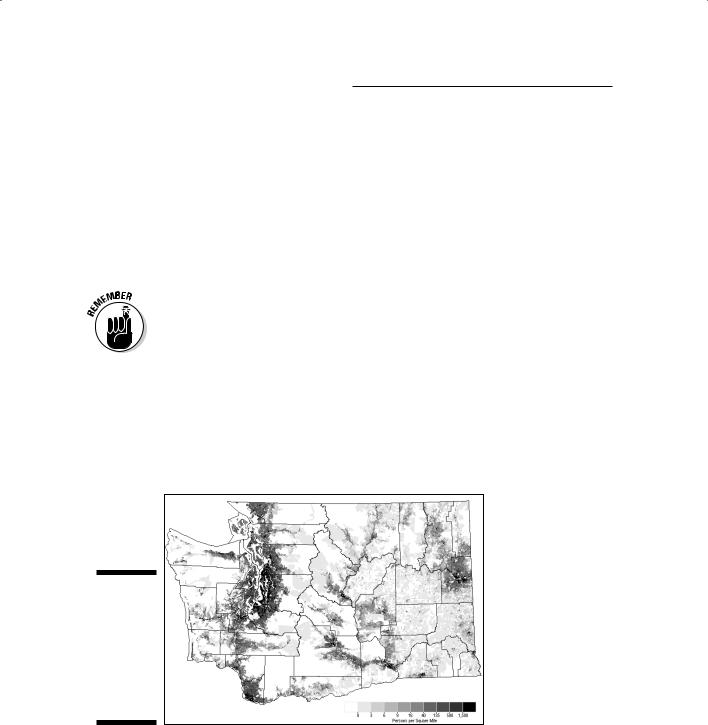
Let me tell you a little secret: If you look carefully at the description of statistical surface properties in the section “Working with Surface Data,” earlier in this chapter, you notice it says, “You can assume that they’re distributed continuously.” That part of the description tells you that the data can be “assumed” to be continuous because, if you suspend your disbelief (pretend they are distributed continuously) for just a bit and wink at the data, you can literally ignore the more rigid part of the definition that says they must be continuous. So, you can display and analyze maps of population distributions (discrete data) just as if people really did occur everywhere, as shown
in Figure 13-6. This assumption of continuity doesn’t cause a problem because even truly continuous surfaces are composed of a discrete subset of sample points, rather than a potentially infinite number of points.
Figure 13-6:
Using a gradient display to map discrete population data as a continuous surface.

Chapter 13: Working with Statistical Surfaces 209
Predicting Values with Interpolation
You can easily figure out the word interpolation if you just look at the first part — in. When you interpolate, you try to predict or estimate missing values in-side a set of numbers by using numbers on either side of the gap. Interpolation is based on the idea that numbers occur in a predictable fashion or sequence. You could fill in this sequence easily — 10, 20, 30, ??, 50, 60. You come up with the value 40 because the numbers don’t occur randomly; they exhibit a sequence (each number is 10 more than the previous number).
Surfaces’ values change in sequences. These sequences determine the way you predict the missing value. Some sequences for surfaces are smooth and steady, and others are rough and undulating. Some sequence of numbers can represent each of these types of surfaces, but the sequence might be very complex. Some sequences might be linear (such as 1,2,3...) and some quite non-linear (for example, logarithmic — rapidly increasing or decreasing curves). The interpolation method you choose depends on the nature of the surface, as described in the following sections.
Determining values with linear interpolation
Linear interpolation is a method of determining missing values that assumes the surface you’re examining changes in a regular, arithmetic progression — such as 1, 2, 3, 4, 5, and so on. Few — if any — natural surfaces satisfy the arithmetic progression. Still, it provides the basis for all the other methods. Essentially, all methods of interpolation are modifications of the linear method based on a combination of both different progressions (number series, such as logarithmic) and advanced knowledge of the surface (knowing how Z values tend to change over distance).
Linear interpolation is simplicity itself. You place a group of elevation values collected by survey or GPS on the map in their exact X and Y locations. From there, you can use linear interpolation to determine the elevation at specific intervals between two endpoints. Follow these steps:
1.Determine the elevation for each endpoint.
In this example, the elevation values are 200 feet at point A and 400 feet at point B, as shown in Figure 13-7.
2.Measure the horizontal distance between the endpoints.
For this example, the distance between points A and B is 1,000 feet.

210 Part IV: Analyzing Geographic Patterns
Figure 13-7:
Linear interpolation.
3.Determine the total change in elevation between the endpoints.
The surface elevation changes by 200 feet (400 feet minus 200 feet) along a distance of 1,000 feet. You assume that the surface elevation for this distance changes in a uniform arithmetic fashion.
4.Specify uniform intervals between the endpoints.
The surface elevation changes by 20 feet for every distance of 100 feet. So, you just need to divide your distance between the two points (A and B) into ten 100-foot chunks.
5.Figure the elevation for the point located at any specified interval.
A point that’s three 100-foot chunks (intervals) away from endpoint A has an elevation of 260 feet, according to this calculation:
starting elevation + (number of intervals × elevation change per interval) =
requested elevation
For this example, you’re looking for the elevation at the third interval from endpoint A:
200 feet + (3 intervals × 20 feet per interval) = 260
feet
|
|
|
|
|
|
|
|
|
|
1000’ |
||||||||||||
A |
|
|
|
|
|
|
|
|
|
|
|
|
|
|
|
|
|
|
B |
|||
elevation |
|
|
|
elevation |
|
|
|
|
|
|
|
|
|
|
|
elevation |
||||||
200’ |
|
|
|
260’ |
|
|
|
|
|
|
|
|
|
|
|
400’ |
||||||
|
|
|
|
|
|
|
|
|
|
|
|
|
|
|
|
|
|
|
|
|
|
|
|
|
|
|
|
|
|
|
|
|
|
|
|
|
|
|
|
|
|
|
|
|
|
100’ |
? |
intervals |
Using non-linear interpolation
Incline ramps are a classic example of a linearly changing surface. I’ve seen many natural areas that are very flat and have a gradual surface incline, but even the most uniform of these areas has imperfections and places where the surface changes in a different way than the majority of the surface. Because you can’t assume that natural surfaces are linear, you need to find methods of interpolation that are non-linear.