

GIS For Dummies
.pdfChapter 16: Comparing Multiple Maps 251
Suppose that you want to do an overlay of a land-use map from 1974 and another from 2004 that contains soil capability class polygons. You want to decide whether the land uses in 1974 were appropriate by looking at whether those uses persisted through 30 years and worked with the soil capability classes. You can perform a series of individual overlay operations, or you can run the comparison based on a set of rules that you establish. This table includes a few hypothetical examples of combinations that you might want to make with your current scenario.
Input Layer 1 |
Input Layer 2 |
Input Layer 3 |
Output Category |
Cornfields 1974 |
Cornfields 2004 |
Suitable for |
Sustainable |
|
|
agriculture |
agriculture |
Cornfields 1974 |
Urban 2004 |
Suitable for |
High energy use |
|
|
urban |
replacement |
Cornfields 1974 |
Abandoned 2004 |
Unsuitable for |
Unsustainable |
|
|
agriculture |
agriculture |
|
|
(ponding) |
|
Wheat fields 1974 |
Fallow 2004 |
Suitable for |
Sustainable |
|
|
agriculture |
agriculture |
Abandoned 1974 |
Cornfields 2004 |
Suitable for |
Sustainability |
|
|
agriculture |
unclear |
Use selective overlay when you have specific combinations that you want to examine but don’t want to create a separate overlay for each.

252 Part IV: Analyzing Geographic Patterns

Chapter 17
Map Algebra and Model Building
In This Chapter
Using cartographic modeling
Getting the hang of map algebra
Understanding the map algebra language and functions
Creating a model
Going live with your model
Testing to make sure that your model makes sense
If you started reading this book here, you’re anxious to get started making the GIS work for you. Although retrieving maps and doing all the indi-
vidual analyses are often enough for everyday tasks, every now and then, you want to watch the GIS spread its wings and do something really spectacular. This chapter explains how you can let your GIS really soar.
|
The original ideas and concepts underpinning this chapter are the brainchil- |
|
|
dren of Dr. C. Dana Tomlin and his PhD advisor, Dr. Joseph K. Berry, then |
|
GIS |
at the Yale School of Forestry. Their work has had a lasting and substantial |
|
impact on how you can use GIS to make models with maps. |
||
|
In this chapter, I use the raster model to demonstrate how cartographic modeling works. I also show you the basics of the cartographic modeling language called map algebra, the functions that the language provides, and how map algebra creates powerful models. Finally, I show you how you can test the output from map analysis for accuracy and acceptability.
Creating Cartographic Models
When C. Dana Tomlin developed his original Map Analysis Package (MAP) for his dissertation, he wasn’t thinking about data structures; he was thinking about modeling. He wanted a tool that would allow him to analyze and combine many maps to produce cartographic models through a process he called (what else) cartographic modeling.

254 Part IV: Analyzing Geographic Patterns
Cartographic modeling is an ordered set of map operations designed to simulate some spatial decision-making (making decisions about geographic space) process. The order or sequence of map operations (including creating, combining, and analyzing) is often critical to the success of a cartographic model, and the idea that the result will simulate a spatial decision process is at the heart of a cartographic model. Each map operation follows a carefully thought-out path to model formulation that
Identifies each and every output of the individual map operations
Outlines each step in how the software derives the output
Determines which map layers serve as the information sources with which the software builds the model
|
People use GIS (cartographic) models only as a spatial decision-making sup- |
|
|
port system. This single application seems to limit the utility of cartographic |
|
GIS |
models, so I like to give the whole idea of decision-making a broader definition. |
|
By decision-making process, I mean any process that simulates physical or |
||
|
||
|
human environments and supports a wide host of possible activities, including |
Immediate action: Activities such as planning, where you decide to immediately employ cartographic modeling for practical resolution of real-world problems.
Theoretical studies: Constructing cartographic models that simulate natural or human activities in geographic space, contributing to the body of knowledge by describing how spatial distributions of geographic features relate to other patterns or processes.
Future planning: Information needed for decision-making support can be exploratory (for example, predicting traffic increases at selected locations over the next ten years) and can often lead to eventual decisions and related actions.
You can accomplish cartographic modeling with either a vector or a raster GIS. The operations used in cartographic modeling — map data analysis, and map comparison and combination — don’t need a raster data model to work. Even so, the cartographic model is at its most robust in the raster environment.
Understanding Map Algebra
Every modeling toolkit, whether spatial or aspatial (doesn’t lend itself to mapping), has a set of individual tools. The carpenter has hammers, saws, nails, and many other tools. The computer programmer has a set of expressions, constants, and syntax rules for each programming language. Every set of tools has a set of procedures that controls how the tools are used effectively. After all, you might be able to pound a nail in with a pipe wrench, but you probably get better results if you use a hammer.
Chapter 17: Map Algebra and Model Building 255
The GIS modeling toolkit is quite robust and demands an equally robust set of guidelines for its proper use. Fortunately, Dana Tomlin and his mentor Joe Berry created a set of rules — a modeling language, actually — that continues to provide a powerful structure for cartographic modeling. This language, called map algebra, is loosely based on matrix algebra — but map algebra is both simpler and more structured.
The upper-left corner of Figure 17-1 shows what mathematicians call a matrix of numbers. To add this 2-x-2 matrix to another matrix, you add the upper-left number from each matrix, the upper-right number from each, and the lowerleft and lower-right of each. You get an answer in the form of another matrix (at the upper-right of Figure 17-1).
|
|
|
|
Matrix algebra (addition) |
|
|
||||
|
2 -1 |
+ |
1 |
1 |
= |
3 |
0 |
|||
|
||||||||||
Figure 17-1: |
1 |
3 |
1 |
-1 |
2 |
2 |
||||
|
|
|||||||||
The similar- |
|
|
||||||||
|
|
|
|
|
|
|
|
|
||
ity between |
|
|
|
Map algebra (addition) |
|
|
||||
matrix alge- |
|
|
|
|
|
|||||
bra and map |
|
|
|
|
|
|
|
|
|
|
|
2 |
-1 |
+ |
1 |
1 |
= |
3 |
0 |
||
algebra. |
|
|||||||||
|
1 |
3 |
1 |
-1 |
2 |
2 |
||||
|
|
|
|
|||||||
|
|
|
||||||||
You can do addition and subtraction pretty easily by using matrix math. You compare the locations of the cells one by one. When you need to use more advanced techniques, such as multiplication and division, for matrix algebra, the numbers aren’t compared upper right to upper right, lower right to lower right, and so on. When you work with GIS, this lack of consistency doesn’t help you calculate map values because the locations on the Earth are fixed to their locations. Map algebra simplifies matrix algebra so that the X and Y locations don’t move when you compare the numbers. Figure 17-2 shows how matrix algebra and map algebra differ when it comes to multiplication.
|
|
|
|
Matrix algebra (multiplication) |
|
|||||
|
|
|
|
|
|
|
1 |
|
|
3 |
|
|
|
|
|
|
|
|
|
||
Figure 17-2: |
|
2 -1 |
x |
1 |
= |
1 |
||||
|
|
|
|
|
|
|
|
|||
The dif- |
1 |
3 |
|
1 |
-1 |
|
4 |
-2 |
||
ference |
|
|
||||||||
|
|
|
|
|
|
|
|
|
|
|
between |
|
|
|
Map algebra (multiplication) |
|
|||||
matrix alge- |
|
|
|
|
||||||
bra and map |
|
|
|
|
|
|
|
|
|
|
|
|
2 |
-1 |
x |
1 |
1 |
= |
2 |
-1 |
|
algebra. |
|
|||||||||
|
|
1 |
3 |
1 |
-1 |
1 |
-3 |
|||
|
|
|
|
|||||||
|
|
|
||||||||

256 Part IV: Analyzing Geographic Patterns
Tomlin and Berry saw the usefulness of being able to compare grid cell numbers by using all the power of mathematics. When they created the map algebra language, they recognized that the X and Y locations weren’t just matrix positions, but positions on the Earth’s surface. Each grid cell location for each layer must correspond exactly with its counterpart in all other layers.
The GIS software must also maintain this correspondence between the locations of grid cell values on multiple layers during analysis — each grid cell on one map must be in the same column and row for its corresponding grid cell on another map. Likewise, each operation will need to follow this rule so that the correct grid cells are compared during analysis. Any serious cartographic modeler is very familiar with this modeling language both because it is so powerful and because it has become the industry standard.
The Language of Map Algebra
Map algebra was developed when GIS software typically used the commandline interface, where you actually typed words to get the software to perform its tasks rather than click icons and pull-down menus. Although today’s
GIS typically employs a graphical user interface, map algebra functionality is still tied to the idea of written commands. Map algebra commands have an English-like language structure, with an action verb (what you do to the
map), direct objects (the maps that you retrieve), and a prepositional phrase (describing what you create as a result of the action).
A simple, but typical command might read like this:
Add (action verb) mymap (the object input map) to yourmap (another object input map) for ourmap (the output map)
When executed, this command uses the power of the map algebra mathematics structure. Each grid cell in each location for mymap is added to each grid cell in each location for yourmap to create an output map with the sum of each of these individual operations found in each corresponding cell location in ourmap. This simplified example gives you the basic idea of how map algebra works.
Performing Functions with Map Algebra
You can use map algebra to perform a wide variety of operations that comprise the cartographic modeling process. These operations include issuing commands themselves, determining when and how often commands are issued, determining the nature of the output, and actually performing the

Chapter 17: Map Algebra and Model Building 257
mathematics of the map analyses. Although these map algebra commands used to be part of a command-line system, they exist as part of the graphical user interface of the modern GIS. And so, you work through the graphical interface to apply the map algebra and make your cartographic models.
Exercising control
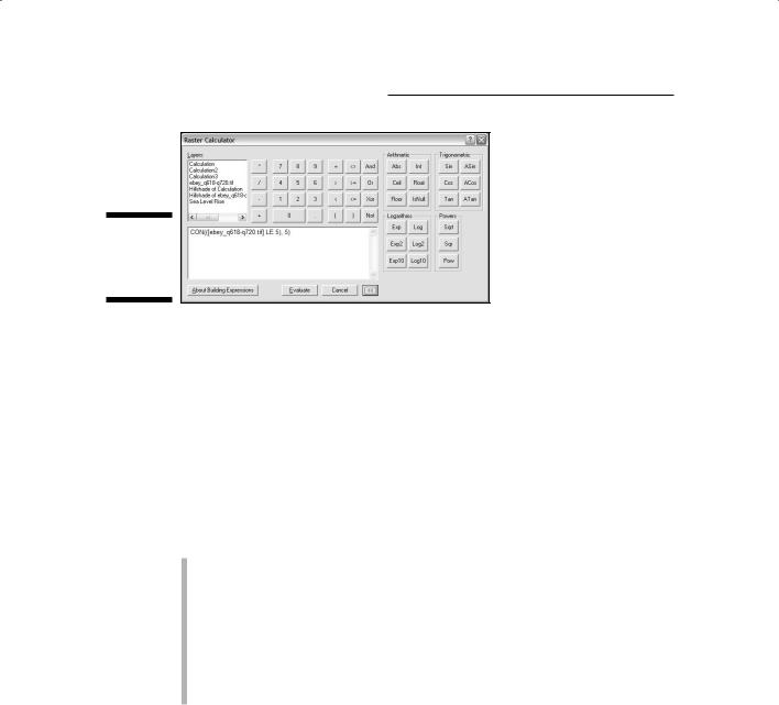
Most of the control you have over cartographic modeling comes from the user interface. A good example of this user interface is the ESRI ArcGIS Spatial Analyst Raster Calculator. This tool allows you to add many types of input to the modeling process, including raster datasets, shapefiles, coverages, tables, constants, and even individual numbers.
This variety gives the software incredible power to shape the model before the software has even done any analysis. The Calculator searches all the data included in the active database and shows the available input data in its search window. You can then query the available data by using the graphical user interface, which you can use much more easily than command-line queries to find what you need.
Besides providing numerous options for input, the Raster Calculator provides a complete set of operators for arithmetic, trigonometric, and logical comparison activities (like most other raster user interfaces do). You can use these operators — which give you access to an extensive set of mathematical manipulations — to create composite groups of modeling tasks called functions.
Essentially, an interface such as the Raster Calculator (shown in Figure 17-3) provides a means to write out complete and often very sophisticated map algebra expressions based on built-in mathematical capabilities. Just a few of these built-in capabilities include addition, subtraction, multiplication, division, roots, powers, absolute values, trigonometric functions, geometric functions, greater or less than, remainders, assignments, and formal logic.
Map algebra expressions that give you control over your model building include
Queries: Find and input data.
Functions: You choose functions based on how you want to compare and analyze the data.
Operators: Direct the mathematical manipulation and logical comparisons to drive the functions.
The power and flexibility of the GIS comes in many different forms in which you can put functions together to take advantage of all the mathematics that the grid cells can use.
258 Part IV: Analyzing Geographic Patterns
Figure 17-3:
The Raster
Calculator
in action.
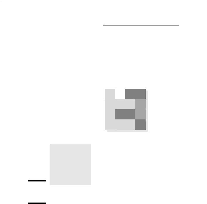
Using local functions
The most basic function type is called the local function because it operates on each cell individually. Sometimes called by-cell operations, these functions are among the simplest — and most often used — of the map algebra functions. Tomlin used to refer to these functions as a worm’s eye view of the grid cells because his theoretical worm could see only a single grid cell at a time and so couldn’t react with other neighboring cells. You can manipulate each grid cell by using virtually any of the operators, and then compare and combine each grid cell with the corresponding grid cells in other layers.
The local functions are usually grouped into six sets of operators:
Trigonometric: Such as sine and cosine
Exponential and logarithmic: Such as squares, cubes, and log base 10
Reclassification: Such as invert, double, and change all to 1
Selection: Such as select all > 2, all between 3 and 10, and so on
Statistical: Such as mean, median, and mode
Other: Mostly mathematical, such as add, subtract, and conditional comparison
Figure 17-4 shows the input grid and resulting output grid after the software applies a trigonometric sine function, and Figure 17-5 shows a statistical example.

Chapter 17: Map Algebra and Model Building 259
|
|
|
1 |
1 |
0 |
0 |
|
|
|
0.8 |
0.8 |
0 |
0 |
|
|
|
|
|
|
|
|
||||||||||
|
|
|
|
|
|
|
|
|
|
|
|
|
|
|
|
|
|
|
|
1 |
2 |
2 |
|
|
|
|
0.8 |
0.9 |
0.9 |
|
|
|
|
|
|
|
|
2 |
|
= |
|
|
|
|
0.9 |
|
|
|
|
|
4 |
0 |
0 |
|
-0.8 |
0 |
0 |
|
|||||
|
|
|
|
|
|
||||||||||
|
|
|
|
|
|
|
|
|
|
|
|
|
|
||
|
|
4 |
0 |
1 |
1 |
|
|
|
-0.8 |
0 |
0.8 |
0.8 |
|
||
|
|
|
|
|
|
|
|
|
|
|
|
|
|
|
|
|
|
|
|
|
|
|
|
|
|
|
|
|
|
|
|
|
|
|
|
Ingrid1 |
|
|
|
|
|
|
Outgrid |
|
|
||
|
|
|
|
|
|
|
|
|
|
|
|
||||
Figure 17-4: |
|
|
|
|
|
|
|
|
|||||||
|
|
|
|
|
|
|
|
|
|
|
|
||||
Local trigo- |
|
|
|
|
|
Value = nodata |
|
|
|
|
|||||
nometric |
|
|
|
|
|
|
|
|
|
|
|
|
|||
|
|
|
|
|
|
|
|
|
|
|
|
||||
functions. |
|
|
Expression: SIN(Ingrid1) |
|
|
|
|
||||||||
|
|
|
|
|
|
|
|
|
|
||||||
|
|
|
|
|
|
|
|
|
|
||||||
If you understand the basic concept of map algebra, you understand pretty much every local function that you can imagine. Local functions are also easier to explain than those that don’t operate on a cell-by-cell basis (such as focal, zonal, and others). You may find the simplicity of these functions handy if you need to explain your GIS modeling to a user.
Using focal functions
Unlike local functions (discussed in the preceding section) — where you zoom in to gain the worm’s eye view — focal functions allow you to pull back a bit and begin to see the area around you. This area is sometimes called
a neighborhood. Focal functions evaluate a single grid cell based on some characteristic of its surrounding cells, or neighborhood. (Focal functions are sometimes called neighborhood functions.) In general, the focal function allows you to look at a target cell (the cell that you’re characterizing or working on), evaluate it based on some relationship it shares with its neighborhood, and return new grid cell value in the same X and Y coordinates but on a new output layer (as shown in Figure 17-6).
260 Part IV: Analyzing Geographic Patterns
|
1 |
1 |
|
0 |
0 |
|
|
|
|
||||
|
|
|
|
|
|
|
|
|
1 |
|
2 |
2 |
|
|
|
|
|
|
2 |
|
|
4 |
0 |
|
0 |
|
|
|
|
|
|
|
|
|
|
4 |
0 |
|
1 |
1 |
|
|
|
|
|
|
|
|
|
|
|
|
|
|
|
|
|
|
Ingrid1 |
|
|
|
|
|
|
|
|
|
|
|
0 |
1 |
|
1 |
0 |
|
|
|
|
||||
|
|
|
|
|
|
|
|
3 |
3 |
|
1 |
2 |
|
|
|
|
|
|
2 |
|
|
|
0 |
|
0 |
|
|
|
|
|
|
|
|
|
|
3 |
2 |
|
1 |
0 |
|
|
|
|
|
|
|
|
|
|
|
|
|
|
|
|
|
Ingrid2 |
|
|
||
1 |
0 |
0 |
|
|
2 |
= |
|
|
0 |
0 |
2 |
|
|
0 |
Outgrid |
|
|
|
1 |
0 |
0 |
|
|
|
|
|
|
|
|
|
|
2 |
0 |
3 |
3 |
|
|
|
|
|
|
|
|
|
|
0 |
0 |
3 |
2 |
|
|
|
|
|
|
|
|
|
|
1 |
1 |
|
0 |
|
|
Value = nodata |
|
|
|
||||
|
|
|
|
|
|
|
Figure 17-5:
Local |
Ingrid3 |
|
|
statistical |
|
functions. |
Expression: MAJORITY(Ingrid1, Ingrid2, Ingrid3) |
|
Focal neighborhoods are based on a search radius and a shape for the search, often called the geometry. Initially, focal functions assume that most neighborhoods include grid cells that border or touch the target grid cell. The neighborhood can, and usually does, extend beyond these bordering cells and can ignore some bordering cells based on the search geometry.