GIS For Dummies
.pdfChapter 17: Map Algebra and Model Building 261
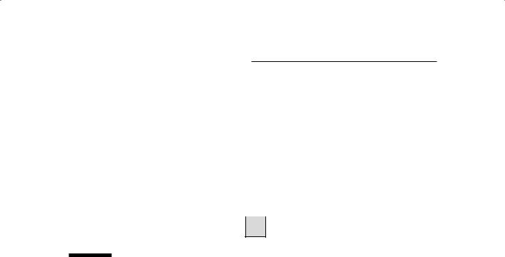
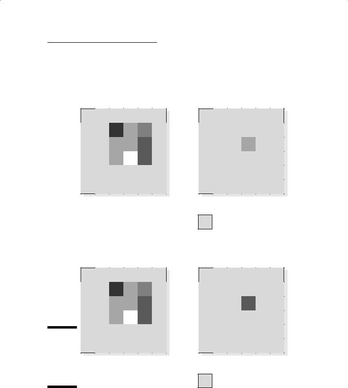
The Neighborhood Function on an Individual Neighborhood
|
3 |
2 |
0 |
|
2 |
2 |
4 |
|
|
1 |
= |
|
2 |
4 |
|
Figure 17-6: |
|
|
|
Focal func- |
|
|
|
tions focus |
|
|
|
on a single |
|
|
|
cell and its |
Ingrid1 |
|
|
relation- |
|
||
|
|
|
|
ship with its |
|
|
|
neighbors. |
|
|
|
4 |
Outgrid |
Value = nodata
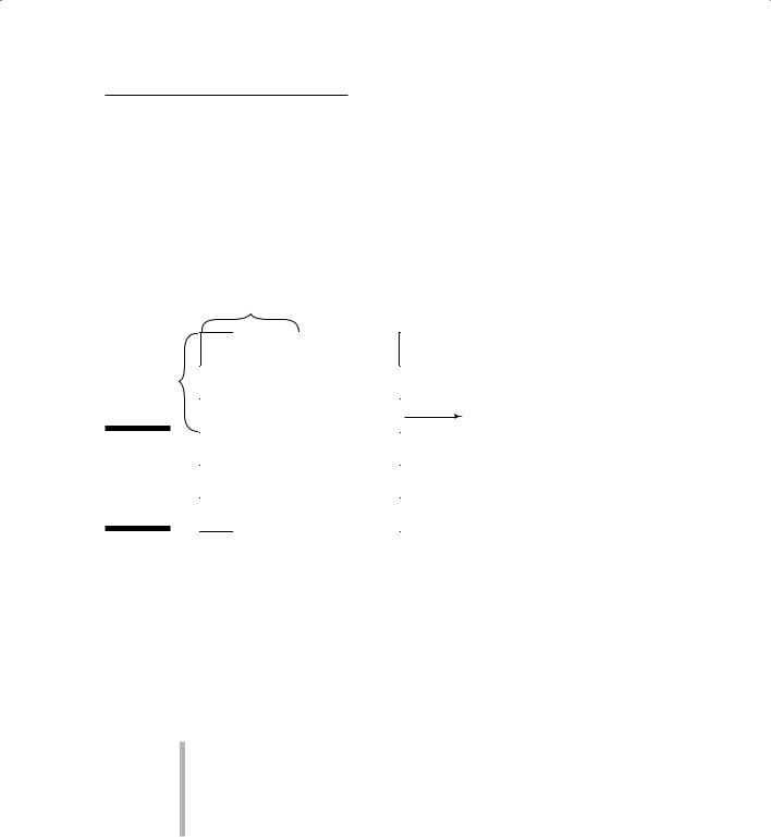
Defining your neighborhood’s size and shape
To create a simple search pattern, search for the eight neighboring cells around your target cell in a 3-x-3 matrix. That configuration is called an annulus (donut shape) with a search radius of one cell (as shown in Figure 17-7). An annulus could search two cells away from the target, three cells, or more.
The Neighborhood Function on an Individual Neighborhood
3 |
2 |
0 |
|
2 |
2 |
4 |
0 |
2 |
1 |
4 |
= |
|
|
|
|
|
|
|
|
|
|
|
|
|
|
|
|
|
|
|
|
|
Figure 17-7: |
|
|
|
|
|
|
|
|
|
|
|
Ingrid1 |
|
|
|
|
Outgrid |
|
|
The annulus |
|
|
|
|
|
|
|
||
|
|
|
|
|
|
|
|
|
|
neighbor- |
|
|
|
|
|
|
|
|
|
hood. |
|
|
|
|
|
|
Value = nodata |
|
|
|
|
|
|
|
|
|
|
|
|
|
|
|
|
|
|
|
|
|
|
262 Part IV: Analyzing Geographic Patterns
You can also evaluate neighborhoods that include rectangles of all nine cells (including the target cell), wedges (pie shapes) in different directions, and circles (including the target cell). In short, you can choose from a few different geometries to define your neighborhood search area.
You select the geometry of your neighborhood for focal functions based on how far away from the target cell you need to go to evaluate grid cells. The distance is often a function of how the real environment you are modeling works (for example, how far from a gas leak you might encounter a fire hazard).
Focusing on focal flow
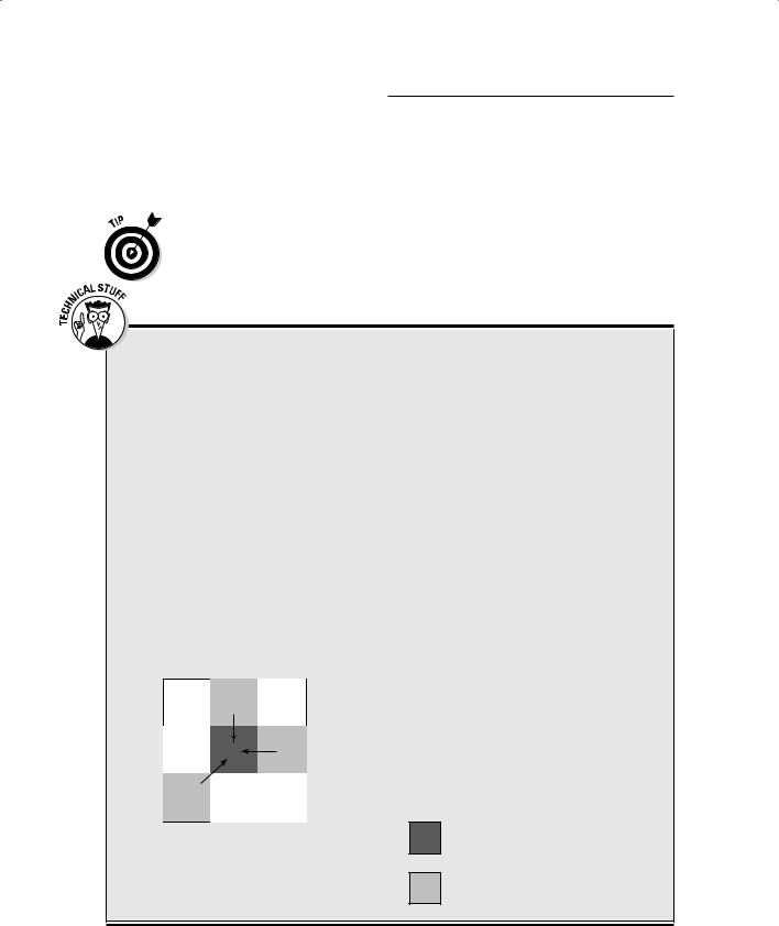
One focal function is called the focal flow function and is really part of the modeling toolkit used for analyzing basins and hydrological conditions (covered in Chapter 14). Focal flow evaluates the neighborhood cells but operates on only the adjacent eight cells — sometimes called the immediate neighborhood. Because of this limitation, you don’t have to tell the software the search radius or the shape.
In most focal operations, the software returns a value to the focal cell (the target of the calculations). This focal flow operation is sort of backwards because it’s really comparing the focal cell to the neighborhood, rather than comparing the neighborhood to the focal cell. You use a focal flow function to determine, given the height of the target cell, which of the outside
cells would allow water to drain (flow) into the target (focal cell).
The GIS compares each height of the neighboring grid cells to the height of the target (center) grid cell. If the neighbor cell is higher, it drains into the target cell. The software puts a 1 into that cell. If the neighbor cell is lower than the target cell, the software assigns that cell a 0. If the neighboring-cell and target-cell values are the same, the software uses one of a variety of different ways to indicate no flow. So, this focal function adds complexity and produces eight values, rather than one, because the software returns values to the neighborhood locations, not to the focal-cell location (as shown in the figure).
-5 |
11 |
3 |
6 |
9 |
15 |
10 |
8 |
8 |
Evaluation for a single cell location
Bit position
8 |
7 |
6 |
5 |
4 |
3 |
2 |
1 |
|
|
|
|
|
|
|
|
0 |
1 |
0 |
0 |
1 |
0 |
0 |
1 |
|
|
|
|
|
|
|
|
Base10 bit values for the cell location = 73
Processing Cell
Cells that flow into the processing cell
Chapter 17: Map Algebra and Model Building 263
You might be scratching your head, wondering how you might need all these different shapes for neighborhoods. Most people will never use all, or even most, of these shapes. Here are a few points about size and shape of impact areas to help you decide on your neighborhood geometries:
The size of your neighborhood area is based on the area of impact of the attributes you’re looking for. Sounds impressive, no? If you know, for example, that people can hear construction noise for ten miles from its point of origin, you can define your neighborhood as a circle with a radius of ten miles.
Circular shapes are common GIS search patterns. The circle is the most compact two-dimensional shape, and is easy to reproduce. The types of features that occur as circles and can take advantage of this circular search methodology are:
•Center-pivot irrigation circles
•Circular animal mounds and ant nests
•Exposed rock domes and salt domes
•Some archaeological sites and Indian mounds
•Coppice dunes
•Crop circles . . . okay, that’s a bit of a stretch — but crop circles exist, no matter who (or what!) creates them
You can search neighborhoods with rectangles because many human features occur in that shape. You’ve probably seen many housing subdivisions divided up into square blocks. You could certainly make a block of a certain size into a neighborhood.
Other shapes can simulate real-world shapes during search. Some shapes are more obscure than circles or rectangles, but some types of features, both natural and man-made, have these kinds of geometries:
•A ring of vegetation around the base of hills, or around ponds and small lakes, forms an annulus.
•Wedges might describe alluvial fans and river deltas, and even the pie-shaped crop types within a single center-pivot irrigation feature.
You can no doubt come up with other characteristics that define your neighborhoods. Each feature that you include in your search provides a reason for you to select the size and shape of your neighborhood. The exact syntax for how you make this selection varies with your GIS software, but essentially, you define the shape and the search size as part of your search strategy.
Comparing your neighborhood to the target cell
After you know the size and shape of your neighborhood (as I talk about in the preceding section), you need to decide what properties you want to use

264 Part IV: Analyzing Geographic Patterns
to compare your neighborhood cells to the target cell. You can use pretty much all the operators you have available in the local functions for focal functions, as well.
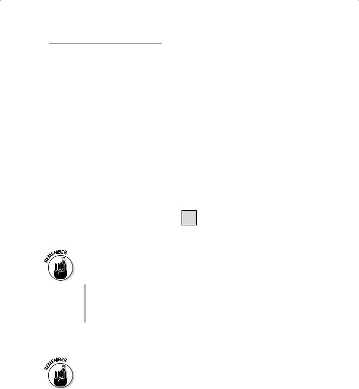
Figure 17-8 shows two simple 3-x-3 annulus examples, one that uses the majority and another that uses the maximum. The first search is a focal majority that returns the number that occurs most often in the annulus to (the eight-cell ring around) the target cell. The focal-maximum search returns the highest number that occurs in the eight-cell ring.
Exploring zonal functions
Unlike focal functions (discussed in the preceding section), zonal functions don’t create neighborhoods. They use zones, either from a single grid or from other layers to compare cells by either attribute (description) or shape (geometry). You need to define the zone with which you want to work. A zone is equivalent to what geographers call formal regions. Regions are areas or groups of areas that share common descriptive information. In a raster data model, a region (or zone) is a group of grid cells that have the same attributes.
Formal geographic regions can be contiguous (all in one chunk), perforated (with holes that have different attributes), or fragmented (like islands that share attributes).
Comparing zonal values
Like with local functions, you can apply a large array of quantitative and logical operators to zonal functions. The most common such operators include majority, minimum, maximum, mean, median, minority, range, standard deviation, sum, and variety.
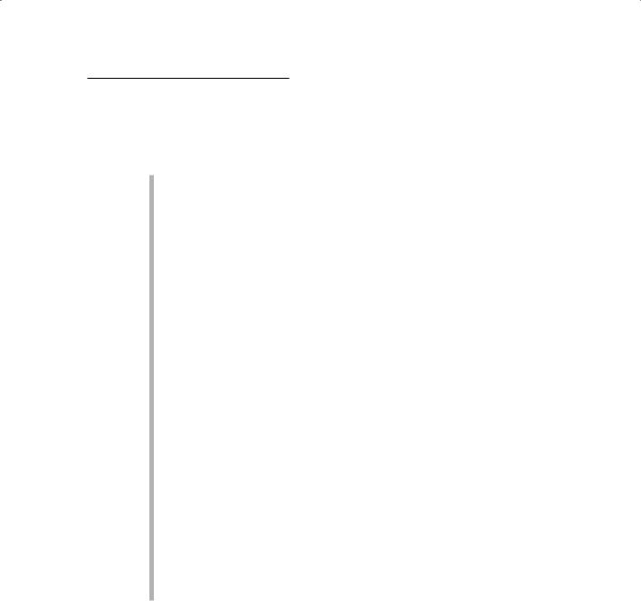
The general approach to zonal functions follows these basic steps:
1.Create one input layer, called the zone layer (Ingrid 1 in Figure 17-9), as the top layer for comparison.
The zone layer defines the zone or zones that you want to evaluate.
2.Create another input layer that has the values you want to use to evaluate for each zone (Ingrid 2 in Figure 17-9).
3.Perform the comparison functions for each zone.
For example, you may want to find the variety for each different zone (as shown in Figure 17-10). Finding the variety tells you which zones (Ingrid 1) have the greatest number of different types of features based on the
Chapter 17: Map Algebra and Model Building 265
grid categories contained in each zone. Ecologists might use this type of function when they want to identify areas of high biodiversity (variety of habitat, for example).
The Neighborhood Function on an Individual Neighborhood
3 |
2 |
0 |
2 |
2 |
4 |
|
1 |
= |
2 |
4 |
|
Ingrid1 |
|
|
2 |
Outgrid |
Value = no data
The Neighborhood Function on an Individual Neighborhood
|
3 |
2 |
0 |
|
2 |
2 |
4 |
|
|
|
= |
|
2 |
1 |
4 |
Figure 17-8: |
|
|
|
The focal |
|
|
|
majority |
|
|
|
(top), and |
Ingrid1 |
|
|
the focal |
|
||
|
|
|
|
maximum |
|
|
|
(bottom). |
|
|
|
4 |
Outgrid |
Value = no data

266 Part IV: Analyzing Geographic Patterns
|
1 |
1 |
|
0 |
0 |
|
|
|
|
|
|
|
|
|
|
|
|
|
|
|
|
|
|
|
|
|
|
||||
|
|
|
|
|
|
|
|
|
|
|
|
|
|
|
|
|
|
1 |
|
2 |
2 |
|
|
|
|
|
|
|
|
|
|
|
|
|
|
|
2 |
|
|
|
|
|
|
|
|
|
|
|
4 |
0 |
|
0 |
|
|
|
|
|
|
|
|
|
|
|
|
|
|
|
|
|
|
|
|
3 |
|
3 |
2 |
|
2 |
|
|
4 |
0 |
|
1 |
1 |
|
|
|
|
|
|
||||
|
|
|
|
|
|
|
|
|
|
|
|
||||
|
|
|
|
|
|
|
|
|
|
|
3 |
2 |
|
2 |
|
|
|
|
|
|
|
|
|
|
|
|
|
|
|||
|
|
|
Ingrid1 |
= |
|
|
|
|
|
||||||
|
|
|
|
|
|
|
|
|
|
|
|||||
|
|
|
|
|
|
3 |
|
2 |
2 |
|
2 |
|
|||
|
|
|
|
|
|
|
|
|
|
|
|
||||
|
0 |
1 |
|
1 |
0 |
||||||||||
|
|
|
|
|
|
|
|
|
|
|
|
||||
|
|
|
|
|
3 |
|
2 |
3 |
|
3 |
|
||||
|
|
|
|
|
|
|
|
|
|
|
|
||||
|
3 |
3 |
|
1 |
2 |
|
|||||||||
|
|
|
|
|
|
|
|
|
|
|
|
||||
|
|
|
|
|
|
|
|
|
|
|
|
||||
|
|
|
|
|
2 |
|
|
|
|
|
Outgrid |
|
|
||
|
|
0 |
|
0 |
|
|
|
|
|
|
|||||
|
|
|
|
|
|
|
|
|
|
|
|
|
|||
|
|
|
|
|
|
|
|
|
|
|
|
|
|
|
|
|
3 |
2 |
|
1 |
0 |
|
|
|
|
|
Value = nodata |
|
|
||
|
|
|
|
|
|
|
|
|
|||||||
|
|
|
|
|
|
|
|
|
|
|
|
|
|
|
|
|
|
|
|
|
|
|
|
|
|
|
|
|
|
|
|
|
|
Ingrid2 |
|
|
|
|
|
|
|
|
|
|
|
||
Figure 17-9:
Zonal
functions.
Expression: ZONALMAX (Ingrid1, Ingrid2)
Classifying zones based on zonal geometry
Zonal functions augment their analytical techniques by allowing you to classify based on the geometry of the zones themselves. This technique works well for finding individual polygons or groups of polygons of a particular size, as shown in Chapter 10. The most common approaches to classification based on zonal geometry include zonal area, zonal perimeter, and zonal thickness. You may find zonal thickness really useful if you’re looking for long and skinny features, for example.
Figure 17-11 shows an example of the zonal area approach, where the software finds and selects zones base on adding up the areas of all the grid cells in each zone. The software then returns the area value to every cell in the zone.
|
|
|
1 |
1 |
|
0 |
0 |
|
|
|
|
|
|
||||
|
|
|
|
|
|
|
|
|
|
|
|
|
1 |
|
2 |
2 |
|
|
|
|
|
|
|
|
2 |
|
|
|
|
4 |
0 |
|
0 |
|
|
|
|
|
|
|
|
|
|
|
|
|
|
4 |
0 |
|
1 |
1 |
|
|
|
|
|
|
|
|
|
|
|
|
|
|
|
|
|
|
|
|
|
|
|
|
Ingrid1 |
|
|
|
|
|
|
|
|
|
|
|
|
|
|
|
0 |
1 |
|
1 |
0 |
|
|
|
|
|
|
||||
|
|
|
|
|
|
|
|
|
|
|
|
3 |
3 |
|
1 |
2 |
|
|
|
|
|
|
|
|
2 |
|
|
|
|
|
0 |
|
0 |
|
|
Figure 17-10: |
|
|
|
|
|
|||
|
|
|
|
|
|
|
|
|
A zonal |
|
|
|
|
|
|
|
|
|
|
|
|
|
|
|
|
|
variety. |
|
|
3 |
2 |
|
1 |
0 |
|
|
|
|
|
|
|
|
|
|
|
|
|
|
|
|
|
|
|
Ingrid2