

GIS For Dummies
.pdfChapter 15: Working with Networks 231
identifies more than one path that they can use to escape. British-designed road systems provide another classic example of circuits with their intersection roundabouts. In the United States, the interstate bypass system allows you to travel around major urban areas without dealing with slower intraurban traffic.
When you perform traffic analysis for routing, allocating customers or bus riders, or finding the nearest facility, having circuits greatly increases your route options. In some cases, the routes may be longer but could save travel time because of reduced traffic and less traffic-related impedances.
Measuring and modeling circuits
The algorithm for modeling circuitry is very similar to the one you use for network connectivity (which I discuss in the earlier section “Measuring and using connectivity”). Rather than a gamma index, you use another ratio called the alpha index. In transportation geography, the alpha index is used to characterize the amount of circuitry. The alpha index, like the gamma index, is a ratio. In the alpha index, the ratio compares the actual number of circuits (loops in a network composed of nodes and links) divided by the maximum circuits possible. Like with the gamma index, both general and transportation-specific GIS software has the alpha index built in for you.
Although you may find having an index of circuitry handy to characterize areas, GIS users more commonly use networks for traffic-pattern analysis. You treat the loop just like any other connection inside the GIS. So, these loops provide alternatives for movement, and you don’t have to do any additional work to set them up or model with them.
Open network |
Closed circuit |
Figure 15-3:
A circuit; also called a closed loop.

232 Part IV: Analyzing Geographic Patterns
Working with Turns and Intersections
Whether your network database has circuits or just different sets of branches, you sometimes must turn or cross another branch that intersects your path. You have to make some turns at right angles, some at acute angles, and some at obtuse angles. You may even encounter a link that meets a dead end or a T that offers two possible directions. These different types of linkage provide an array of alternative movements that the GIS can handle.
Recognizing the importance of turns and intersections
When you plan a trip, you need to know where you’re starting, where you’re going, what the traffic will probably be like, which roads or streets you must take, and where you turn from street to street. Some routes may require you to travel more distance than other routes. Some routes have stoplights that slow your movement. Although your map may not show it, some streets are one-way streets — and those streets might lead to your destination or might flow one way in the wrong direction. Turning from two-way streets to oneway streets means that the turns themselves also restrict your movement by forcing you into specific lanes on which you can travel.
Stoplights, stop signs, and different types of street intersections all either add or detract from your travels. Planning a trip means more than just looking at the lines on a map and tracing the shortest route. One time-saving trick I like to use is to plan a trip where I make only right-hand turns. Experience has taught me that cutting across traffic (with left-hand turns) can be difficult and time-consuming because you must wait for an opening to get across.
Because you no longer have to rely on a static, hardcopy road map, you can include knowledge about what factors speed travel and what factors slow it down when you travel along a road network. The more compete this information, and the more accurately it represents how intersections and turns work, the more likely you can accurately model traffic. The key to successful traffic network modeling, then, is getting all the right information into the computer.
Encoding and using turns and intersections
You can code turns for any junction where edges connect. The number of edges connecting at each junction limits the number of possible turns. The maximum number of turns is the number of edges n squared, or n2. You can

Chapter 15: Working with Networks 233
even model a single edge where your maximum number of turns is one, (12 = 1). Figure 15-4 shows graphically how this formula works with a T intersection composed of three links.
When you have three links (or edges), squaring that number tells you that you have nine possible movements, including U turns and straight-through (non-turn) movements, as follows:
Three U turns: Each edge provides an opportunity to do a U-turn if you allow it.
Two right turns and two left turns: The link coming down from the top allows you to make right turns along the inside lane, and left turns to the outside lane.
Two non-turns: The links on the bottom allow you to go straight through, or turn into the vertical link from the right or the left, depending on your approach.
Turns are defined by rules that affect conditions in which two edges come together. Every GIS employs some set of rules that govern how and where you can make turns. These rules will likely reflect the terminology used in your GIS software package, but, in general, GIS turn rules give you these restrictions:
You can’t set up turns that include impossible movements or seriously violate traffic laws.
You can create U-turns, but you can turn that ability off if, for example, U-turns aren’t legal.
Some software stores turn information as network datasets, and others use turn tables that include a field for adding a turn impedance (see the section “Working with Impedance Values,” earlier in this chapter). Turn impedance values, which network datasets also include, give you the opportunity to include the amount of time it would normally take to perform a turn with traffic or against it. So, you can model vehicular movement very realistically.
|
|
U-turn |
|
|
|
Left |
|
Right |
Figure 15-4:
The possible turns in a T
intersection.
Straight transition

234 Part IV: Analyzing Geographic Patterns
Directing Traffic and
Exploiting Networks
Networks provide a selection of really useful techniques that you can employ in businesses, government, organizations, emergency services, and many other applications. After you add to your GIS a complete network that has appropriate road designations and ID codes for your impedance values, the impedance values themselves, plus turn information, you have one of the most powerful networking tools available anywhere. Here’s a quick list of the operations you can use in most GIS software:
Finding the best route (shortest, fastest, or even the most scenic)
Finding the closest geographic feature to you
Finding service areas, such as what parts of town are served by a single fire station
Finding the shortest path, or route
Many people use street maps to figure out the shortest route from their current location to some specified location. If you search for the shortest path, you use the length of the network links to decide the best route. Because you’re not concerned with time, you don’t need to include impedance values in your search. Although the GIS ignores most impedance values when you specify that they aren’t needed, the software always includes some indication of one-way streets and dead ends so that it doesn’t send you on a wild goose chase.
Most GIS use several algorithms to determine the shortest path, but most of these algorithms look at a number of alternate routes and choose the shortest. One common method of shortest path search is called the best first algorithm, which takes the shortest path available at each step. Other algorithms try a number of alternatives at predetermined distances and select the best.
Consult your software documentation for more detail, but most of these techniques provide pretty good results.
Even if you don’t own a complete professional GIS, you may have already seen this ability to find the shortest path in action. Yahoo! Maps and Google Maps find the shortest path from one town to another or one address to another. These packages are rudimentary GIS software and do a reasonable job for general routing tasks. For detailed, time-critical routing, especially for business and emergency services, these packages typically don’t include the detail that you need to efficiently navigate through road networks, especially during critical times of the day like rush hour.
Chapter 15: Working with Networks 235
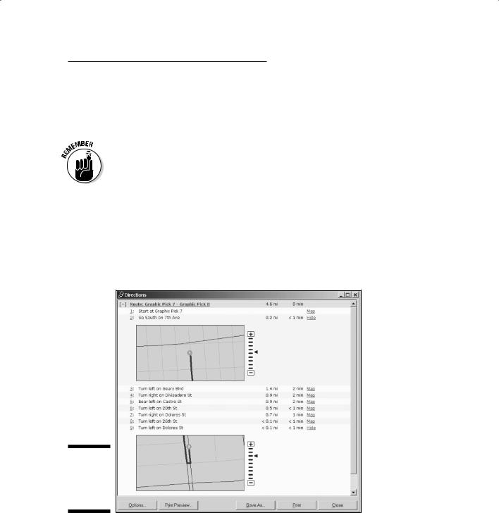
Both the rudimentary packages and the more sophisticated GIS software provide two forms of output. The first form is a map that shows a highlighted version of the route. You can expand this map to a turn-by-turn map that includes a text version of exactly how far each leg of the route is, exactly where the turns are, and which direction you turn (like the example in Figure 15-5).
The shortest path means shortest in terms of distance traveled. If you want to get there fast, use the fastest-route feature of your GIS (see the next section for more on this feature).
Finding the shortest route to one destination is pretty handy, but you can also use the GIS to find the closest of a group of possible destinations, as well. You’ve probably used this kind of feature when you wanted to find the closest Sears or Wal-Mart store by using the store’s Web site. The software finds the addresses of all the possible locations and performs a shortest-path analysis on all of them from your current location. Businesses have found that providing interactive maps directing traffic to their front door (so to speak) is a really powerful marketing tool.
Figure 15-5:
A turn-by- turn map with the directions.
Finding the fastest path
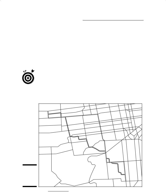
The shortest way from one place to another isn’t always the fastest, as shown in Figure 15-6. For example, you might be able to get from the southeast corner to the northwest corner of a big city much faster by taking the
236 Part IV: Analyzing Geographic Patterns
interstate around the city, rather than taking the shorter diagonal route. The shorter diagonal route includes slow speed limits, traffic congestion, stop signs, stoplights, and a host of other possible impedances.
The fastest-path search allows your GIS to start from one location and accumulate impedance values while it searches through the network to find your destination. Instead of keeping track of just distance, it combines distance and impedance to calculate the route that has the least amount of total impedance. Typically, GIS software measures impedance in time, so a street that has a 25 mile-per-hour speed limit has a higher impedance value (longer time) than one that has a 75 mile-per-hour speed limit.
You can use the fastest-route search method for another useful search. If you know where you’re starting but don’t know your destination, the GIS can find your destination for you. Okay, the GIS isn’t going to find the perfect picnic spot or the best restaurant unless you give it a clue. Perhaps you have a sick family member and you need to get him or her to the hospital. If your town has four or five hospitals, the GIS can search for the closest one. You need to tell the software that you want it to find the fastest path to all the selected hospitals in your area and the fastest of those is the one you would select.
Figure 15-6:
The shortest path versus the fastest path.
Fastest Path |
|
Shortest Path |
|
Chapter 15: Working with Networks 237
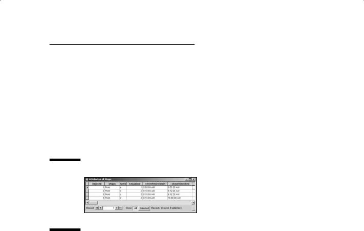
One aspect of the fastest-path approach is a bit unique because your impedance values are based not just on speed limits, impedances, and typical traffic volumes, but also on the time of day. Some construction zones operate at different times of day, traffic congestion is worse during rush hours, and even the season might impact which roads are open. Encode in the OD matrix the times of day when traffic is congested on which streets to make sure that the software can determine how drivers can avoid those streets at those times. In some hilly cities and towns, selected streets are blocked off at times in winter because the snow and ice make those streets dangerous to drive. You can code all sorts of impedances as windows of time along selected portions of the network and store them in an attribute table, as shown in Figure 15-7.
Figure 15-7:
Setting up a time window table in the ESRI ArcGIS network module.
Finding the nicest path
You may be concerned about factors other than speed or distance. Many highways have scenic routes that are a bit slower or perhaps even longer than a more direct route, but you may want to view the scenery. GIS software can help you find the scenic routes, as well as the fastest and most direct routes, because you can create scenic impedance values. When you run your search, you simply ask the GIS to search for links that have the nicest scenery. You just need to remember to include the values that you want to search for in your network database attributes.
Finding the service areas
The network database allows you to create all sorts of values to put into your tables. You can include distance, impedance, turning, and even scenic information. One really powerful tool for service providers and businesses alike is the ability to find service areas.
A service area identifies places that are within a reasonable distance for use and relies on knowing how many people or houses are located along individual links in a network, much like impedance values, except that the database has to know how many people are along each link. The software starts
238 Part IV: Analyzing Geographic Patterns
at some point location and searches either along a chosen path or outward in all directions. While it searches, it counts all the houses or people it passes until it reaches the end of the database, some specified search radius, or some maximum quantity of people or houses.
 You may find the service area tool useful in a number of different settings. GIS Here’s a list of some common uses:
Creating bus routes for school children, limiting the search by the number of passenger seats on the bus
Determining how many fire stations a town needs, based on a search of the number of homes one fire station can safely service (based on historical numbers of fires and other factors) in a worst-case scenario
Marketing to potential newspaper subscribers based on an accumulated search of households that don’t currently subscribe to your paper
Creating service areas in which a pizza delivery store can deliver pizzas within an assigned time period
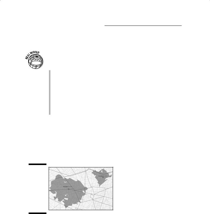
Figure 15-8 shows the results of a search that returns all areas in a portion of a city that a driver can reach within five minutes. Service-area analysis allows you to use all the impedance and turning tools that you use for any other analysis. This process of finding service areas, often called allocation
by geographers, is a very popular tool among business analysts because they can not only allocate for their own facility, but also compare themselves to their competition. Allocation is one of the more popular economic placement tools available in GIS today.
Figure 15-8:
The results of servicearea analysis showing areas that are reachable within five minutes.

Chapter 16
Comparing Multiple Maps
In This Chapter
Looking into map overlay
Comparing polygons with logical overlay
Understanding the advantages of raster overlay
Using selective overlay to compare features
Geographers have been aware for generations that spatial patterns sometimes repeat themselves. The usefulness of comparing these
spatial patterns has been documented as far back as the Revolutionary War when General George Washington’s French cartographer made multiple hinged maps that showed the locations of both British and American armies in the corresponding geographic area. This idea probably goes back as far as maps themselves.
In the early 1960s, the idea of using computers to make maps brought with it a renewed interest in comparing multiple map patterns. Landscape architects used clear acetate to physically overlay and compare maps manually with a fair degree of success. Urban and regional planners found comparing different maps essential to the observation, quantification, explanation, and eventual exploitation of multiple patterns.
Even before map overlay came into use, people observed patterns occurring in the data contained on various maps for an area. Auto thefts happen in locations that have cars, shopping happens in areas that have stores, roads connect towns, vegetation responds to different soil types and different slopes, cities mostly occur near water, certain wildlife prefer selected vegetation, people of similar income tend to live in the same areas, and so on. You can observe each of these coincident patterns both in the field and on maps. You can analyze the degree to which the patterns correspond, and figure out whether cause and effect relationships exist, much more easily if you can overlay the maps.

240 Part IV: Analyzing Geographic Patterns
This chapter shows you the three main ways to compare multiple maps. I show you how you can use mathematics and formal logic to make the comparisons. You see how overlay works in raster and vector data models, and how to use selective overlay to compare particular features across maps.
Exploring Methods of Map Overlay
The ability to overlay maps was a primary driving force during the early development of GIS software. Initially, overlay functions focused on comparing one set of polygons to another, but they quickly expanded to comparing polygons with point and line features. For people, overlaying one map on another is a pretty simple concept involving a visual and intellectual interpretation process. But getting a computer to do the overlay is a bit more complicated because the interpretation process can take several forms and may even combine different methods. Fortunately, you don’t need to worry about these details because the methods have been formalized into some very structured approaches in the GIS software.
All professional GIS software has some form of overlay toolkit that allows you to choose among different methods of overlay and select the layers you want to use. Most GIS toolkits have a separate graphical user interface or offer a button, icon, or tool to click that, in turn, gives you a lot of choices. Check your user manual or type help overlay in your software’s help utility.
Knowing the overlay methods available helps you find the right tools in your own software. Map overlay operations compare three pairings of geographic feature types:
Points to polygons
Lines to polygons
Polygons to polygons
The first two pairings, points to polygons and lines to polygons, use a presence/ absence overlay method. In other words, either the points or lines coincide with (occur in or run through) a particular type of polygon or they don’t. This method is actually a little more complicated than that (as I explain in the following sections), but not much.
The last pairing — polygon to polygon — introduces some additional potential methods of comparison that, to some degree or another, simulate the intellectual process of visual map overlay. Each method is adapted to either raster or vector GIS data models, as I describe in the following sections.