

GIS For Dummies
.pdfPart IV
Analyzing
Geographic
Patterns

In this part . . .
The most advanced functions of GIS lie in the systems’ capacity to measure geographic features, including
distances, areas, networks, surfaces, and all their related characteristics. In this part, you find out how GIS performs individual tasks, such as finding shortest or fastest routes, analyzing visibility, assessing fluid accumulation and flood zones, and many others. Also, you discover how to combine these individual operations to create complex, real-world models, which are (in my opinion) the most rewarding pinnacle of the GIS analyst’s art and science.

Chapter 12
Measuring Distance
In This Chapter
Measuring absolute distance
Calculating relative measurements
Figuring out distance based on function
You can measure anything you put on a map. You use map measurements to figure out how far you are from one place or another, how much land
you own, how much ore you might expect to get from a new mine, and many other measurements. You can measure heights, widths, depths, lengths, areas, and volumes. You can also compare measurements as ratios — for example, ratios of length to width, perimeter to area, or height to distance.
Measuring geographic features is one of a GIS’s strengths, and it does the measuring very quickly! Because you can measure many features quickly, you can use those measurements to help you make decisions about what route to take (by comparing distances between features), whether one place is better than another for mining (by calculating the volume of a specific feature), or where you’re likely to find the best ski slopes (by evaluating a feature’s height against its length).
In this chapter, I show how GIS gives you the power to measure all sorts of features. First, I explain the measurements that GIS software generates by default (such as grid cell size), and then I describe how the GIS uses these numbers to calculate other measurements (such as distance between objects). I also tell you about the difference between relative and absolute measurements, and when you might want to use each. I explain how you can use measurement tools to describe how features are distributed relative to each other and to other surrounding features. And finally, I describe how to apply distance to make entirely new polygons based on the distances you measure.
Taking Absolute Measurement
When you enter data into a GIS, the software keeps records of those points, lines, and polygons. More important, it keeps a record of the X and Y locations
184 Part IV: Analyzing Geographic Patterns
of your vector or raster objects. It stores the size of the grid cells and the lengths of the lines. Having these records saves a lot of time when you calculate distances.
The measurement of absolute distances, whether between objects or along lines, is computed differently for raster and vector data structures. The following sections describe these measurement methods and how the computer implements them for both data types.
Finding the shortest straight-line path
Finding the shortest straight-line path between any two points is the simplest method to measure distance. Often called “as the crow flies” distance, this Euclidean method makes two assumptions:
1.No obstructions block the path between the two points.
2.You don’t need to travel along established paths and roads.
The following sections describe how the GIS software enables you to find the shortest straight-line path between two points that exist under a variety of circumstances.
Finding the shortest distance on a flat surface
If you’re working on a flat surface, the shortest distance between any two points (a straight line) is based on a well-known mathematical equation
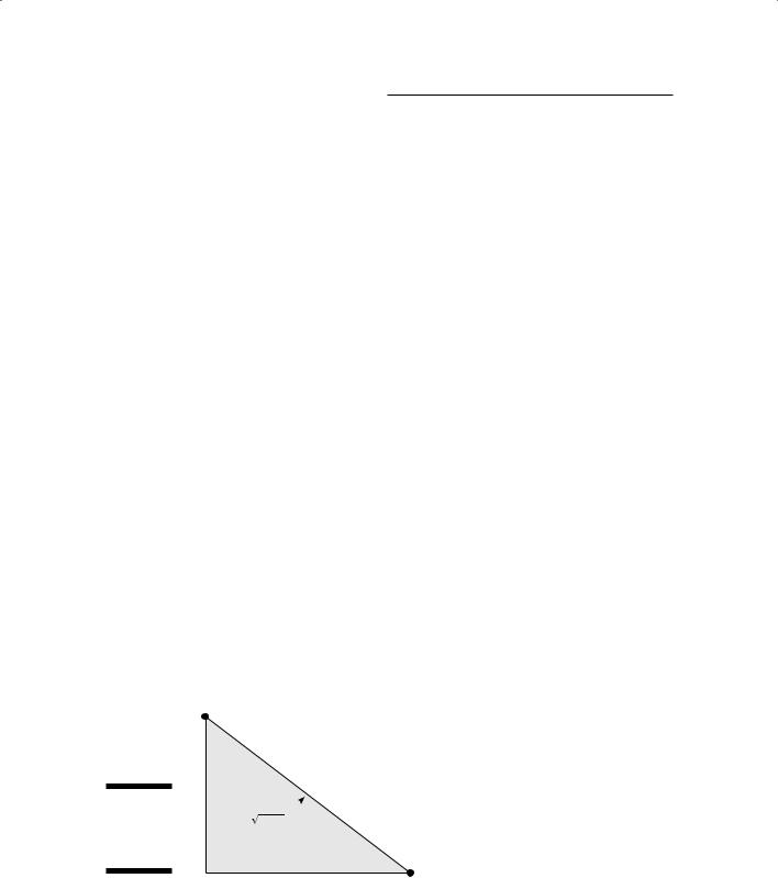
(c2 = a2 + b2), the Pythagorean Theorem (named after the ancient Greek mathematician Pythagoras). The Pythagorean Theorem is based on the use of a geometric form called a right triangle — any triangle that has one corner that makes a right-angle turn (90 degrees). The longest side of this triangle, the one opposite the right-angle bend, is called the hypotenuse. Figure 12-1 shows an example of a right triangle.
Figure 12-1:
An example of a right triangle.
5.00 |
Endpoint |
|
4.00 |
LegVertical |
|
3.00 |
||
|
||
2.00 |
|
Hypotenuse |
(7 |
|
|
|
. |
|
81) |
62 + 52 = 7.81
1.00 |
|
|
|
Horizontal Leg |
|
Endpoint |
|
|
|
|
|
||||
|
|
|
|
|
|||
1.00 |
2.00 |
3.00 |
4.00 |
5.00 |
6.00 |
||
Chapter 12: Measuring Distance 185
Remembering sines and cosines
When you work with planar coordinates for measuring distance, you need to know the X and Y values for each point. So, you can convert spherical coordinates to planar coordinates as follows:
The X location: X = r × cos(a) × cos(b)
The Y location: Y = r × cos(a) × sin(b)
Here are what the letters stand for in the preceding transformations:
r: The radius of the Earth
a: The latitude
b: The longitude
Seeing sines (abbreviated sin) and cosines (abbreviated cos) may make your eyes water, but you can remember what these terms mean
by taking the pneumonic device SOHCAHTOA and breaking it into three parts — SOH, CAH, and TOA:
SOH: Sine equals Opposite over Hypotenuse
CAH: Cosine equals Adjacent over Hypotenuse
TOA: Tangent equals Opposite over Adjacent
So, to calculate sines and cosines, you really just have to divide. After you transform all your spherical coordinates to planar coordinates, you can apply the formulas that you use to calculate straight-line distance to your new X and Y coordinates. But I have even better news — the GIS does all this for you!
Each of the two points (that you want to measure the distance between) is defined by an X coordinate and a Y coordinate along number lines. To locate each point, you have to move horizontally and vertically along the number lines from the origin point (where the right angle forms) to the values that define your points. These movements along the number lines define the straight legs of your right triangle. You can think of the distance between those two points as the hypotenuse of your right triangle.
When measuring real Earth distances in a GIS, the software calculates the hypotenuse distance using the X and Y values of two points in a modification of the Pythagorean Theorem called the distance formula. You’ll encounter this distance formula many times in your GIS work.
When you need a quick online refresher on the distance formula, visit www. purplemath.com/modules/distform.htm.
Finding the shortest distance on the spherical Earth
The GIS can also calculate distance between a set of latitude and longitude coordinates on a spherical Earth. You may need to find the shortest distance between two points on the globe. This calculation is called a great circle distance and uses a geographic grid. The calculation of latitude and longitude distances has some very strong similarities to calculating distance by using
186 Part IV: Analyzing Geographic Patterns
flat (planar) coordinates and the distance equation. (In Chapter 2, I describe a bit about converting a spherical Earth to its representation on a flat piece of paper.) This process, called map projection, involves mathematics because it converts spherical coordinates to planar coordinates.
Conversely, no space on the Earth is totally flat, so calculating the distance between any two points requires some determination of the spherical coordinates. Your GIS is already set up to perform these calculations for you. Using trigonometric formulas and the X and Y (planar) coordinates of geographic features, your software can easily change back and forth from spherical geometry to planar geometry. If you really want a peek at the math behind this conversion, check out the sidebar “Remembering sines and cosines.”
Measuring distances in grid cells
Measuring distances in raster systems (using grid cells) is a bit different than measuring distance in vector systems, both conceptually and computationally. Many raster GIS packages allow you to calculate measurements in both flat coordinate systems and the geographic grid (latitude and longitude coordinates). The alternative to measuring by coordinates is counting up grid cells.
If all the grid cells in the path you’re measuring are edge-to-edge (orthogonal), you can easily figure the distance the path covers. Just count up the grid cells and multiply that number by the width of the grid cell. For example, if you count 150 grid cells from one point to another and each grid cell is 20 meters across, the total distance is 20 × 150, or 300 meters.
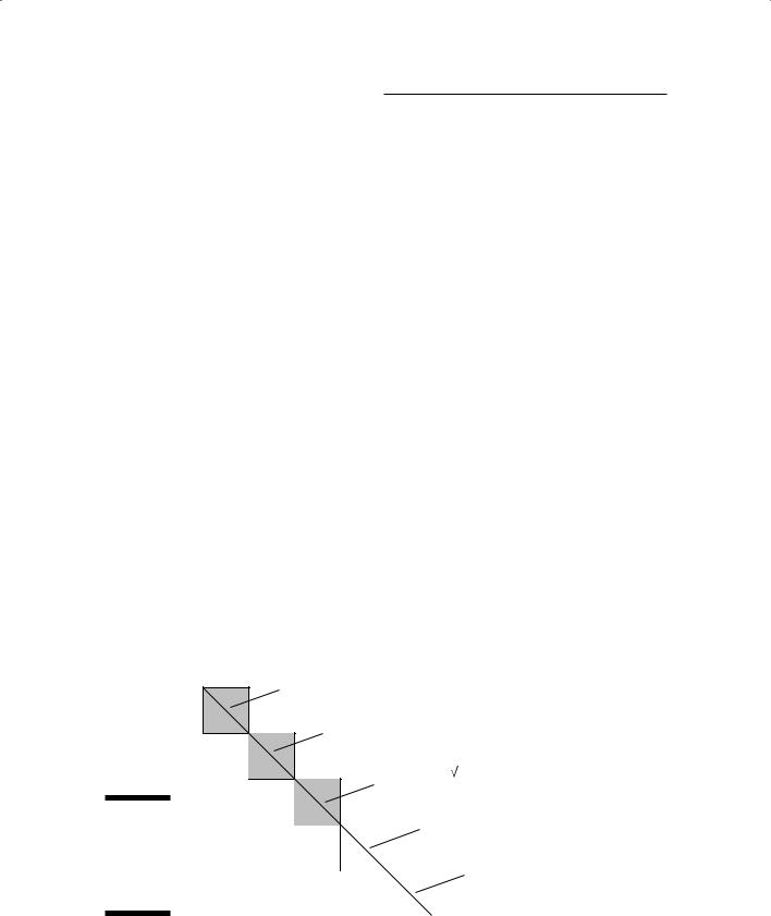
This very simple approach gives you pretty accurate results, but only if all the grid cells are orthogonal or all distances are exactly lined up by the cardinal directions. In real distances, you seldom get such an exact configuration. If you’re working with a raster system in which you want to measure distances that are diagonal, you need to measure grid cells that are diagonal to one another, at least for some portion of the distance (as shown in Figure 12-2).
Figure 12-2:
Measuring diagonal distance in grid systems.
|
c=1.414 |
|
|
a=1 |
|
|
|
b=1 |
1.414 |
c2=a2+b2 |
|
|
|
||
|
c2=1+1=2 |
||
|
|
||
|
|
c= |
2=1.414 |
|
|
1.414 |
|
.Total |
1.414 |
||||
7 |
|
|
|
||
07 |
|
|
|
|
|
UnitsLength |
|
|
1.414 |
||
= |
|
|
|
|
|
|
|
|
|
|
|
Chapter 12: Measuring Distance 187
Measuring Manhattan distance
When I was a young lad in Minnesota, I used to like to go through large department stores on my way home to get out of the stinging cold and, ideally, shorten my path. But actually, the path I took was just as jagged as if I’d stayed outside. Although I did manage to warm up for a few minutes, I probably didn’t make my trip any shorter.
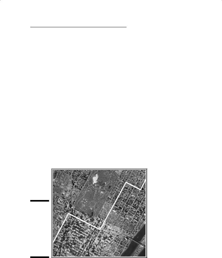
Imagine you’re in the downtown business portion of any large city, such as New York City’s Manhattan, where the streets are laid out like a grid. Each block is the same size, and tall buildings prevent you from moving anywhere but along these blocks — unless you can leap tall buildings in a single bound, of course. Likewise, cars must follow the streets that separate these blocks. The distance from point A to point B, unless both points are on the same block, is going to be longer than if you could travel “as the crow flies,” as I discuss in the section “Finding the shortest straight-line path,” earlier in this chapter. Because Manhattan is an excellent example of this restricted movement, geographers refer to distance measurements in this environment as
Manhattan distance.
Figure 12-3 shows a hypothetical city with the same type of structure as downtown Manhattan. To travel from point A to point B, you need to follow the edges of the blocks. By moving along the blocks, you have to travel a much larger distance than if you could travel the straight-line distance. This grid structure allows many possible paths from one point to another, but each path covers essentially the same distance.
B
Figure 12-3:
Measuring
Manhattan distance moves from point A to point B along
an unob-  A structed
path.
188 Part IV: Analyzing Geographic Patterns
To calculate Manhattan distance, you use a modification of the distance equation, but conceptually, the calculation is really much simpler than that. Because each of the edges for each block is a straight line segment, you need to know only where the X and Y coordinates are for the ends of each line segment. Most GIS software automatically stores that information when you first input the data. You can easily calculate each line segment’s length using the distance equation included in the GIS software. To determine the total Manhattan distance, you simply let the software add together each individual line segment’s length.
Calculating distance along networks
You encounter many types of routes in GIS work — including footpaths, animal tracks, rail lines, intercity roads, and street patterns — that look nothing like Manhattan. Each of these networks typically indicates an imposed structure on distance traveled. To calculate distance along these networks, the GIS measures vector segment lengths or grid-cell lengths for vector and raster, respectively.
Vector: The GIS first retrieves the X and Y coordinates of each line segment’s endpoints (stored at input) and then uses the distance equation to determine each line segment’s length. Finally, the GIS adds together all the individual line segment lengths.
Raster: The GIS finds each orthogonal grid cell’s width and then adds those to get the total length. When grid cells are diagonal to each other, the lengths are measured as the width multiplied by 1.414 (the diagonal distance of a grid cell), as illustrated in Figure 12-2.
You can measure linear features in raster, but you can both represent and measure features more accurately in vector.
In Manhattan distance, you don’t gain anything by choosing a different route. With most irregular networks, however, you can choose many routes from point A to point B, and these routes often have wildly different distances. Your software can measure all these possible routes and find the one that has the shortest distance by using the shortest path algorithm (an algorithm is like a recipe to solve a problem). Chapter 16 covers the shortest path algorithm in more detail.
Working with buffers
Nearly all GIS software has a set of special distance functions designed to selectively calculate distances around existing geographic features. These operations are called buffering (no, not like the aspirin), and the result is
Chapter 12: Measuring Distance 189
called a buffer. The software measures outward a certain distance from a point, line, or polygon (even the base of a topographic feature), and it then converts that whole area to a polygon.
A lot of real-world features contain buffers — prescribed, natural, or enforced distances that surround them:
Easements around power lines, railroads, and so on
Road frontages and street setbacks
River vegetation, beaches, and drainage-way vegetation
Police lines, safety zones, and concert barricades
Earthquake zones and 100-year flood zones
The user bases each corridor on rules, natural occurrences, safety, utility, security, and any number of other factors. The GIS allows you to implement these conditions and rules in a number of different ways, as described in the following sections.
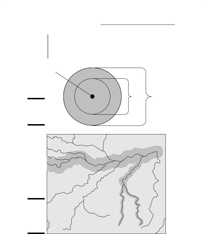
Placing buffers around points
You can place buffers around point objects, such as wellheads. You can decide to make this type of buffer either a single distance measure or in multiples (as shown in Figure 12-4). So, if you put a buffer around a wellhead as a safety corridor, you can actually create several levels of safety corridor — 100, 200, and 300 meters, for example. These might be classified as modest, medium, and high risk based on a safety officer’s experience.
Placing buffers around lines and polygons
Buffers around lines and polygons give you three options that point buffers don’t:
Variable buffer: By using the GIS variable buffer function, you can select the size of the barrier for each portion of a line or polygon feature, instead of being forced to use the same-sized buffer for the entire feature. For example, in a river network, the trunk stream probably has more vegetation on it than its tributaries do, so it has a larger corridor than its tributaries’ corridors (see Figure 12-5).
Setback buffer: You can determine whether a buffer will be the same size on either side of a feature. In some cases, this difference is extreme — the buffer exists on only one side of a feature. This type of buffer is called a setback buffer because it’s “set back” in only one direction. You can position a setback in either direction from a line feature (for example, the center of a street). For polygon features, the setback buffer is usually established (set back) from the perimeter to some distance inside the feature.
190 Part IV: Analyzing Geographic Patterns
Bidirectional buffer: Most buffers measure distance outward. Setback buffers can measure distance inward. One advantage of doing a buffer around an area feature is that you can have a buffer going both directions at once. Most GIS software allows you to select this option so if you want to measure a buffer distance both inward and outward from the outside perimeter of an area feature, you can.
Point
Buffer 1 |
Buffer 2 |
Figure 12-4:
You can create buffers around points.
Figure 12-5:
This variable buffer surrounds a river’s trunk and tributaries.
80 mile buffer
 Amazon
Amazon
Tapajos
40 mile buffer
20 mile buffer |
Rio |
|
Teles |
||
JuruenaRio |
||
Pires |
||
|
20 mile buffer |