

GIS For Dummies
.pdfChapter 13: Working with Statistical Surfaces 211
Non-linear methods of surface interpolation try to match the numeric progressions they use to the progressions that most closely approximate how the surface changes. To most effectively decide which of these non-linear interpolation methods to employ, you need a close understanding of the nature of the surface, including both
A conceptual idea of how the surface looks before you map it
A working knowledge of what factors influence how the surface might react to changes in other factors.
When selecting a non-linear interpolation method, first characterize your surface (gradual, steep, or a combination; smooth, rugged, or some combination). Then, become familiar with the nature of the processes at work that cause the surface to exist. With this knowledge, you can match the techniques that best suit the way the surface changes.
Estimating values with distance-weighted interpolation
The weighted-based-on-distance method is more properly called inverse distance weighting. The closer things are to each other, the more likely that they’re related. So, if you have a bunch of numbers (say from GPS data) that you can use to interpolate missing data, the numbers that are closest to the missing data probably have more meaning. This method gives a higher weight to closer values and less weight to those that are farther away. This
type of interpolation method (weighted) is one of a growing number of methods called exact interpolation methods.
Here are some examples of how distance to something affects its importance for interpolation:
If you need to purchase a single candy bar, do you go to the local convenience store just down the street or travel the 8 miles to the supermarket, where you might save a nickel or a dime?
Do you talk to your friends who live 1,000 miles away as much as you talk to the people who live in your immediate neighborhood?
Your favorite music group is having a concert next week 500 miles away, but the same group will be in your city next month. Are you more likely to go to the concert at home or 500 miles away?
You can always find exceptions to these examples, but generally, the closer you are to your candy bar, your friends, or your favorite rock band, the more likely you are to interact with them.

212 Part IV: Analyzing Geographic Patterns
The same idea applies to surface data. Consider temperature data. If you’re standing at one place where the temperature is 75 degrees Fahrenheit and you take a step to your left, you expect that the temperature is pretty close to 75 degrees in that location, as well. But if you get in your car and travel 100 miles from your original location, you probably don’t expect to find the same temperature at your destination.
Knowing the other exact interpolation methods
You use exact interpolation when you can’t take the risk of assuming a linear change in Z value. The word exact means that many parameters are taken into account, such as the relationships of distance to weight of the interpolation. Some exact interpolation methods require the user to define search radiuses. Other interpolation methods don’t require the user to define radiuses. Some interpolation methods calculate the point at which distance has no effect on interpolation (meaning that no relationship apparently exists between the surface values that are so far apart).
You can find a comprehensive list of interpolation methods here:
www.spatialanalysisonline.com/output/html/
Comparisonofsamplegriddingandinterpolationmethods.html
The table that you find at this site lists the interpolation method, speed, type, and comments that can assist you in deciding which of these methods to use.
I find a particular method — called polynomial regression, or more commonly, trend surface — quite useful for making surface generalizations. This method doesn’t provide an exact prediction of missing values but deviates from exactness to give a general idea of how the slope is trending. You can use this kind of trend surface method if you just want a general idea of a surface — and
the accompanying general trend in a distribution — rather than all the gory details.

Chapter 14
Exploring Topographical Surfaces
In This Chapter
Using topography to identify what you can and can’t see
Working with stream basins
Understanding the relationship of topography to flow
Identifying the parts of a stream
Topography deals with the configuration of the Earth’s physical surface and landforms, their characteristics and locations, and their graphic
depiction on maps. Topographic surfaces can be flat and uniform, or deeply dissected by streams and their associated watersheds or drainage basins (areas that drain in the stream). Some topographic surfaces are gentle and rolling, moving fluids slowly, and others are rough and steep, causing fluids to move rapidly with great erosive force.
You can find a staggering number of forces that create diverse land surfaces, as well as different surface types. Fortunately, earth scientists have grouped, summarized, and generalized most of these forces and their resulting effects to produce some pretty substantial models that you can use. In this chapter, I show you three basic groups of models based on topographic surfaces: viewshed analysis, basin analysis, and stream morphometry (stream shape analysis).
Modeling Visibility with Viewsheds
Analyzing terrain so that you can identify places that are (and aren’t) visible from a known location on the earth is called viewshed analysis. Just like a watershed is a place where you can find the presence of water, a viewshed is a place where you can observe an object in your line of sight. You can analyze visibility from two perspectives:
214 Part IV: Analyzing Geographic Patterns
Point to point: Analyze visibility from one point to another point. You have to know the location of your target point (the place you do or don’t want to see) and the location of the observation point where you (the observer) are standing.
Multiple locations to multiple locations: What if you aren’t staying in one place? For example, say that you plan to walk along a mountain trail and you want to make sure that — during your walk — you don’t see the housing development in the area. Unlike point to point analysis, you determine the visibility of multiple locations along the path to multiple parts of a housing development. Same problem, same solution — just more computing.
The importance of viewshed analysis
You can use the ability to determine what you can and can’t see from selected locations in many ways. Military planners use this technology so that they can place their troops and equipment in places that are hidden from as many locations as possible. Some telecommunications systems require line-of-sight analysis so that they can properly place their transmission equipment. In urban areas, city planners like to hide the unsightly highways from residents’ view; viewshed analysis helps determine where to apply terrain and even vegetation surfaces to solve the problem. In many cases, obscuring the view also produces a quieter environment. For example, Department of Transportation (DOT) workers erect barriers that both obscure and quiet the sound of large highway systems.
Viewshed analysis can tell users where they can see things and where they can hide things from view. If you subtract from the map the area that you can see, you’re left with the area that you can’t see. One area is the complement of the other. Here’s a list of some additional possible ways that you might use viewshed analysis:
You want to build a resort retreat that’s obscured from the city but provides a mountain view.
You’re putting up billboards along a curvy highway, and you want motorists to see the billboards for the longest time possible.
You need to know where to place cellular towers so that as many people as possible get good reception.
You want to know the best place to put your military forward observers so that they get the best possible view of the battlefield.
You need to set up fire watch stations that see both over the topography and over the trees.
You may find viewshed analysis helpful in any number of applications. Just ask yourself these questions:
Chapter 14: Exploring Topographical Surfaces 215
Will the terrain affect whether I can see certain features?
Do I want to see those features or not?
Then, let the GIS work its magic.
Using ray tracing
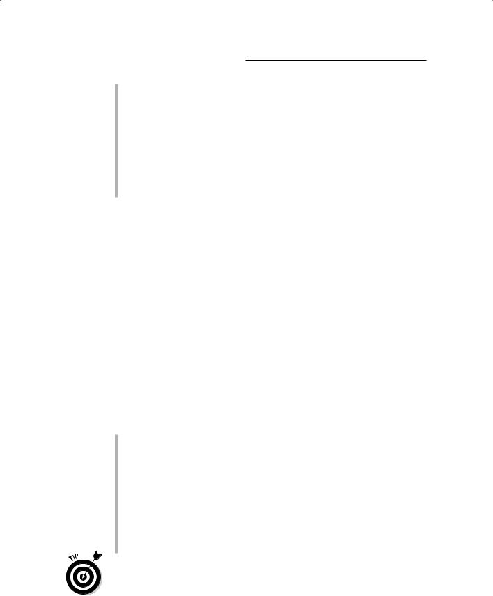
When you look at topography, you can easily imagine a line drawn from each of your eyes to each point in the landscape they view. These lines are identical to the lines that physicists work with in the study of optical geometry (the graphical portrayal of the properties and behavior of light from place to place using lines to show how light interacts with objects it encounters). They draw lines from a subject’s eyes, through lenses, and to and from viewed objects. GIS viewshed analysis uses the same technique. The GIS draws lines from the observer to the observed. GIS users call this technique ray tracing. The GIS software is literally tracing a line from your observer to
different locations on the map. Figure 14-1 shows ray tracing in action. Notice how the line drawn from the observer to a point on the surface shows places that are visible and those that are hidden from sight (shaded).
Figure 14-1:
Simulating line of sight with ray tracing.
Line |
of |
Sight |
|
||
|
|
Not Visible
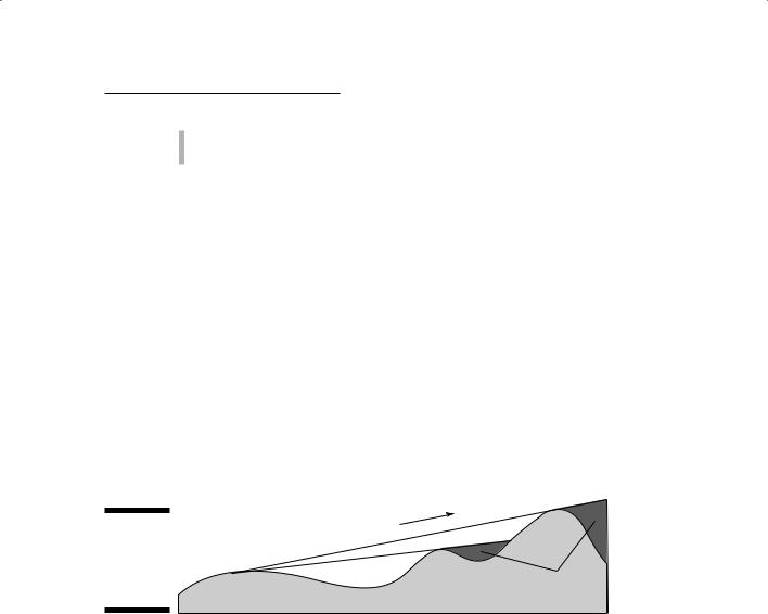
You can use ray tracing to analyze one line of sight at a time, but you typically assess visibility for all possible locations everywhere within the map. By comparing one or more observer locations with all other locations, the software defines the visible and hidden polygons from a potential observer. You can examine visibility over a surface by creating a complete viewshed, such as the one in Figure 14-2, but you may also want to make this even more realistic.
The simple approach assumes that you, the observer, are on the ground and that you’re searching your topography to see what you can see. This approach usually employs only a single layer to analyze, and that layer is normally a topographic layer such as a Digital Elevation Model (DEM). The real world is a bit more complicated than this model would suggest, unfortunately. Real landscapes have trees, buildings, and other obstructions. Plus,
when you observe terrain, you don’t normally lie flat on the ground with your eyes at ground level.
216 Part IV: Analyzing Geographic Patterns
You can easily build these little surface features into your viewshed model. If you’re the observer and you’re standing, your eyes are probably anywhere from 4 to 6 feet off the ground, depending on your height and the shoes you’re wearing. So, if you’re working with a topographic model and have
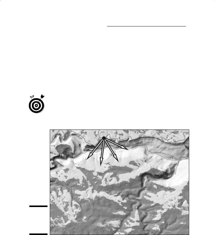
no vegetation or buildings to get in the way, you need to adjust only for the height of your eyes from the ground. To make that adjustment, you just add that height value — say, 5 feet — to the observer’s elevation. If you’re observing from a tall building or a lighthouse, add that additional height to the existing elevation at your observer’s location. You also account for obstructions such as trees in the exact same way. Just add their heights to their locations’ elevations. Figure 14-3 shows the line of sight for an elevated observer and or when obstructions block the way.
The most accurate viewshed models add the heights of obstructions from data in other map layers, as well as from the observer’s height. Most of the time, though, you don’t know the observer’s height, and your elevation model isn’t accurate enough for these minor improvements to make a huge difference. Use these refinements only when you have very good elevation data and a thorough knowledge of the observer and the obstructions.
Figure 14-2:
A viewshed, where the light areas are visible.
Chapter 14: Exploring Topographical Surfaces 217
Obstruction
Figure 14-3: |
|
|
Make |
|
|
adjustments |
|
|
for observer |
|
|
elevation |
|
|
and |
|
|
obstruc- |
Elevated |
|
tions. |
||
Observer |
||
|
Finding and Using Basins
You can find analyzing stream configuration useful for characterizing the flows along these networks (as I talk about in Chapter 15), but you can do much more with the terrain models inside your GIS. For example, you can analyze what the watershed or basin within which your streams reside actually looks like. The basin determines the nature of your stream, and the basin also controls water accumulation (which I discuss in the section “Working with basins in your GIS,” later in this chapter).
These three metrics — stream ordering, basin analysis, and water accumulation — are all inextricably linked to one another. You can’t really do stream ordering until you can define the stream based on a thorough knowledge of the basin. When you have a complete model of the basin, you can finally model the movement and accumulation of water.
Knowing how basins work
Think about what happens in a basin, whether a washbasin or a stream basin. When water enters the basin from above, that water immediately begins to seek its way downhill because of gravity. Water acts differently, depend-
ing on whether a basin is steep or shallow. Steep basins tend to have really sharp cuts in them because the water is moving so much faster than it does in a shallow basin and therefore cuts deeply into the surface. The software must define the movement of water based on the shape of the basin. You usually begin with a set of elevation data from some source, such as a Digital Elevation Model (DEM).

218 Part IV: Analyzing Geographic Patterns
Basins or watersheds are composed of the area upslope from the stream network in such a way that all the water landing on the watershed could potentially flow overland into that stream network.
Working with basins in your GIS
To define both streams and the basins in which they reside, you must first develop a grid (set of grid cells) that illustrates where the water would accumulate if you filled the basin with water. The accumulation is really a measure of distance based on where the water will go. The deeper the basin, the deeper the potential water accumulation. These deep areas are near the central trunk stream (the large stream in the center). Shallow parts of the basin are typically near the tributaries (the branches from the central stream) because water accumulates through movement from tributary streams and from overland flow.
Like with all topographic surfaces, a basin (a low landform associated with a stream network) can include many little depressions and peaks. The GIS can model these differences but the process is unnecessarily complicated. In this discussion, I pretend that my surface has no minor variations. This depressionless surface allows for the development of a general model. You can most effectively model stream basins by using a raster GIS, as I do in this section.
After building your topographic database, you can create a model of the grid surface. The highest grid cells — the ones on the outside margin of your basin — define the basin’s boundaries. The section “Finding and quantifying streams,” later in this chapter, discusses how the lowest grid cells for each sub-basin (a part of the basin associated with a tributary stream) form the cells that make up the stream network. The places where the stream grid cells form each sub-basin are called pour points because, at these locations, water pours from one sub-basin to another.
You want to identify the location of the watershed boundaries mainly so that you can model the accumulation of water while it flows downslope into the basin itself. While you move from the highest elevations, each grid cell contributes water to the total water moving downslope. Because each grid cell downslope receives the water from the grid cell above, the values accumulate.
The more grid cells upslope, the larger the values at the bottom (as shown in Figure 14-4). The left part of the diagram shows the elevation values, the right shows the direction the flow will move based on those values. The GIS records these directions as a series of codes (shown at the bottom of Figure 14-4) based on direction. So, for example, a flow to the right would be coded a value of 1, a flow to the left would be 16, and so on.
Chapter 14: Exploring Topographical Surfaces 219
78 |
72 |
69 |
71 |
58 |
49 |
|
|
|
|
|
|
74 |
67 |
56 |
49 |
46 |
50 |
|
|
|
|
|
|
69 |
53 |
44 |
37 |
38 |
48 |
|
|
|
|
|
|
64 |
58 |
55 |
22 |
31 |
24 |
|
|
|
|
|
|
68 |
61 |
47 |
21 |
16 |
19 |
|
|
|
|
|
|
74 |
53 |
34 |
12 |
11 |
12 |
|
|
|
|
|
|
2 |
2 |
2 |
4 |
4 |
8 |
|
|
|
|
|
8 |
2 |
2 |
2 |
4 |
4 |
|
|
|
|
|
|
|
1 |
1 |
2 |
4 |
8 |
4 |
|
|
|
|
|
|
128 |
128 |
1 |
2 |
4 |
8 |
|
|
|
|
|
|
2 |
2 |
1 |
4 |
4 |
4 |
|
|
|
|
|
|
1 |
1 |
1 |
1 |
4 |
16 |
|
|
|
|
|
|
|
Elevation |
|
Flow Direction |
Figure 14-4: |
32 |
64 |
128 |
16 |
|
1 |
|
Basin accu- |
|
||
mulation. |
8 |
4 |
2 |
|
|||
|
Direction Coding |
||
In this simplified version of how the accumulation model works, each grid cell usually has additional attributes that include values such as the amount of precipitation, and absorption rate of the surface over which the water moves. These values are similar to the friction values that you use when you measure functional distance, as discussed in Chapter 12. The GIS can include these values for more sophisticated modeling operations by adding both the cells and the friction values while the accumulation proceeds.
Characterizing Flow
Watersheds are pretty irregular in elevation values, even if you ignore the occasional highs and lows in the surface. These irregularities result in water moving in different directions. When you add differential surfaces to your GIS database, you can build some really powerful models of flow direction. The following sections show you the basics of how flow direction works.
Knowing the importance of flow
The direction of the movement of liquids downhill determines where erosion is likely to take place, how quickly the water will move, and the moving water’s possible destructive force if important structures happen to be in its path. People build many structures in floodplains and basins. While water
220 Part IV: Analyzing Geographic Patterns
moves down slopes, it not only increases in speed and force, it also saturates surfaces, dislodges portions of those surfaces, and picks up debris that contribute to the potential for damage.
Modeling and using flow
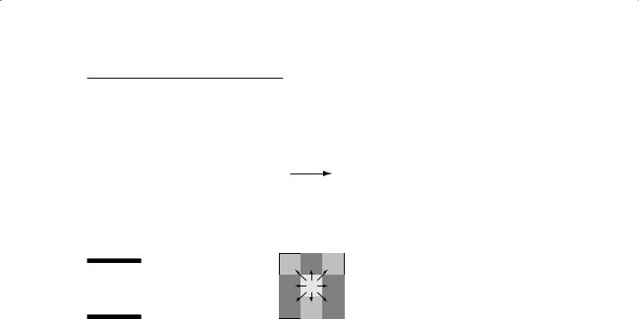
To determine flow direction, you need a grid of elevation values, such as a Digital Elevation Model (DEM). You evaluate each grid cell by comparing its elevation value to that of its neighbors. In Figure 14-5, the GIS compares each of the outside grid-cell elevation values to the center (target) cell. After it determines which cell has the highest drop in elevation, it assigns that cell a code that indicates the direction of water movement.
|
|
145 |
|
132 |
|
112 |
|||
|
|
|
|
|
|
|
|
|
|
|
|
|
|
|
|
|
|
|
|
|
|
|
|
|
|
|
|
|
|
|
|
|
|
|
|
|
|
|
|
Figure 14-5: |
|
137 |
|
|
103 |
|
|
142 |
|
A nine-cell |
|
|
|
|
|
||||
|
|
|
|
|
|
|
|
|
|
(3-x-3) |
|
|
|
|
|
|
|
|
|
|
|
|
|
|
|
|
|
|
|
grid that |
|
|
|
|
|
|
|
|
|
|
|
|
|
|
|
|
|
|
|
contains |
|
|
|
|
|
|
|
|
|
elevation |
|
139 |
|
142 |
|
141 |
|||
values. |
|
|
|
|
|
|
|
|
|
|
|
|
|
|
|
|
|
|
|
|
|
|
|
|
|
|
|
|
|
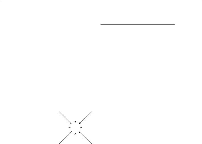
In Figure 14-5, the input grid shows an elevation value for each of the nine grid cells. By using the center grid cell’s value as the starting point (essentially, where the water is at that time) and comparing it to each of its eight neighbors, the computer tries to find elevation values lower than the starting grid cell (in this case, the center). If the elevation values are higher than the starting cell, the computer moves to values that are lower. GIS software packages handle similar surrounding values differently but normally perform a search beyond the immediate neighborhood of cells. The GIS software looks for the direction of steepest descent, meaning the one neighboring grid cell that has the steepest drop in elevation from the starting cell. In Figure 14-5, the grid cell in the upper-left corner has the largest elevation drop to the central grid cell of all the eight neighbors.
To let the computer know that the largest elevation drop is in the upperleft corner, you need to give the flow a direction value. Depending on your software, the eight possible direction values could start on the top, bottom,