

GIS For Dummies
.pdfChapter 2: Recognizing How Maps Show Information 31
GIS
Comparing thematic maps
All things are related to each other in geographic space, but close things are more related than far things. This concept is used frequently in GIS when thematic maps are compared to see what things occur near each other. For example, you can use these maps to do a variety of analyses:
Earthquake hazards
100-year flood zone
Soils with high shrink-swell clay
If, for example, you can locate the zones with the highest frequency of earthquake, your insurance
company can decide whether to issue earthquake hazard insurance, or your builder might have to use some earthquake-proof building techniques to allow for that type of activity. Insurance companies that issue flood insurance need to know whether their potential customers live within an area that’s likely to flood frequently. The building contractor would find a soils map that shows high shrink-swell clay useful so that he or she knows whether to add pylons to reinforce that new skyscraper to keep it from becoming the next Leaning Tower of Pisa.
The more detail, the more complete the information, and the more precisely located the geographic features, the better the analytical results you can get. You might think that the poorest quality map determines the quality of your analysis. This weakest link hypothesis makes sense on the surface, doesn’t it? In cases where each map layer is of equal importance, this hypothesis might be true. However, in most GIS analysis that you do, the different map layers aren’t equally important. Maps that are poorer in quality may still add value to your GIS as long as their lower accuracy does not affect the overall quality of the analysis.
Working with Projections and Datums
Except for members of the Flat Earth Society, everyone accepts that the Earth is roughly spherical. This spherical shape has some major drawbacks for the mapmaker who’s faced with producing a flat map that correctly represents the shapes, angles, distances, and sizes of objects on the Earth. In simple terms, the conversion from a sphere to a flat map is always going to result in some distortion. Peel an orange and try to flatten the peels on a table; now you have a visual idea of the problem that the mapmaker faces.
32 |
Part I: GIS: Geography on Steroids |
Picking the right projections
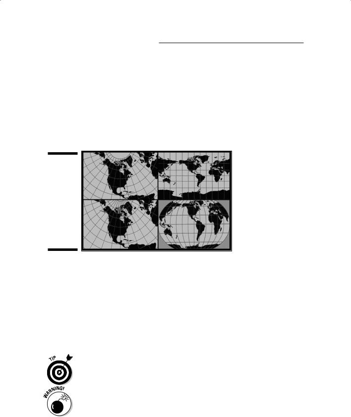
Figure 2-4 shows some of the many ways a map can look. Map projections — the process of converting the spherical Earth to a flat surface — come in many different types, from contiguous to interrupted, from those that look like photographs of the Earth to those placed on cones or cylinders. In fact, cartographers often refer to the three families of map projections as planar, conic, and cylindrical, which describe the surfaces onto which the surface of the Earth would be projected (hence the term projection) if a light bulb could be put in the center of the Earth.
Figure 2-4:
A map can represent a place in many different ways, each of which produces some form of distortion.
The curved surfaces of the Earth just don’t cooperate when you try to make them flat. The mapmaker has to figure out which of the map’s properties he or she most wants to preserve. For maps designed to measure distance, the mapmaker might choose to preserve distance on the map. Another map might be used to determine directions, which requires that shapes be pre-
served. Anyone trying to measure areas or changes in areas wants a map that preserves area.
The good news is that you don’t have to know all the gory details about how the mapmaker preserves certain properties to work with GIS — but you do want to know which properties are mostly preserved.
When working with GIS, pick the map projection that best represents the properties you want preserved when you create output maps from your analysis. For example, if your analysis involves changes in area, a map projection that preserves area is the best type to use to display your results.
Most high-end GIS software has the capability to convert back and forth from one projection to another. Most have more map projections than you’ll ever use. But every time you change from one projection to another, the software

Chapter 2: Recognizing How Maps Show Information 33
rounds off numbers and makes tiny errors in position. If you convert projections repeatedly, these tiny errors in position start to add up. Eventually, you can add enough error to have a negative impact on your analytical calculations.
Good projections depend on accurate datums
The impact of converting projections, like with many other GIS-related transformations, depends on scale. Small scale maps will be affected more than large scale maps. Having an accurate representation of distance and area measurements in any projected map depends on having accurate measurements of the spherical Earth. The science of geodesy deals specifically with these measurements.
Like with any measurement, you need to have a place to start, a baseline. In geodesy, such baselines for measuring the Earth are called datums. In simple terms, the datum is a model of the Earth’s shape that allows geodetic scientists and surveyors to accurately measure the Earth and place the origins and orientation of the coordinate systems.
Each of the hundreds of datums has different measurement units and methods for measuring the Earth. Some datums start by measuring the Earth’s diameter in different directions, others focus on flatness ratios (ratio between the polar and equatorial diameters), and still others are based on measuring the Earth’s circumference at different places Because each datum uses different methods and different models of the Earth (which are called reference ellipsoids), the maps associated with a datum depend on these properties. Table 2-2 gives you an idea of the possible datums you might encounter in your work. You can find a quite exhaustive (or is that exhausting?) list of datums online at
www.colorado.edu/geography/gcraft/notes/datum/datum_f.html
Table 2-2 |
A Few Datums Used in Map Projections |
|
Ellipsoid |
Semi-major axis |
1/flattening |
Airy 1830, |
6377563.396 |
299.3249646 |
|
|
|
Modified Airy |
6377340.189 |
299.3249646 |
|
|
|
Australian National |
6378160 |
298.25 |
|
|
|
Bessel 1841 (Namibia) |
6377483.865 |
299.1528128 |
|
|
|
Bessel 1841 |
6377397.155 |
299.1528128 |
|
|
|
Clarke 1866 |
6378206.4 |
294.9786982 |
|
|
|
Clarke 1880 |
6378249.145 |
293.465 |
|
|
|
(continued)

34 |
Part I: GIS: Geography on Steroids |
|
|
|
|
|
|||
|
|
|
|
|
|
|
Table 2-2 (continued) |
|
|
|
|
|
|
|
|
|
Ellipsoid |
Semi-major axis |
1/flattening |
|
|
|
|
|
|
|
Everest (India 1830)” |
6377276.345 |
300.8017 |
|
|
|
|
|
|
|
Everest (Sabah Sarawak) |
6377298.556 |
300.8017 |
|
|
|
|
|
|
|
Everest (India 1956) |
6377301.243 |
300.8017 |
|
|
Everest (Malaysia 1969) |
6377295.664 |
300.8017 |
|
|
|
|
|
|
|
Everest (Malay. & Sing) |
6377304.063 |
300.8017 |
|
|
|
|
|
|
|
Everest (Pakistan) |
6377309.613 |
300.8017 |
|
|
|
|
|
|
|
Modified Fischer 1960 |
6378155 |
298.3 |
|
|
|
|
|
|
|
Helmert 1906 |
6378200 |
298.3 |
|
|
|
|
|
|
|
Hough 1960 |
6378270 |
297 |
|
|
Indonesian 1974 |
6378160 |
298.247 |
|
|
|
|
|
|
|
International 1924 |
6378388 |
297 |
|
|
|
|
|
|
|
Krassovsky 1940 |
6378245 |
298.3 |
|
|
|
|
|
|
|
GRS 80 |
6378137 |
298.257222101 |
|
|
|
|
|
|
|
South American 1969 |
6378160 |
298.25 |
|
|
|
|
|
|
|
WGS 72 |
6378135 |
298.26 |
|
|
WGS 84 |
6378137 |
298.257223563 |
|
|
|
|
|
Your GIS software needs to know what datum you’re using for each set of map data that you put into your database. Attaching your coordinates to the wrong datum can result in location and measurement errors. You’ll commonly begin with maps that use different datums. To make your GIS data from maps of the same area correspond to each other, they all need to be converted to a common datum.
When loading up your GIS, be sure to use the correct datum for each map source as you add it. Also, convert all your map data to a common datum when you work with more than one source map at a time.
Working with Coordinate Systems and Land Subdivisions
No matter what the theme, projection, or scale, you need to find your way around on your maps — and that’s what coordinate systems help you do. On a globe, you use the latitude-longitude system. On flat maps, you have to

Chapter 2: Recognizing How Maps Show Information 35
convert this geographic grid to something a bit more practical. Ultimately, all coordinate systems are based to some extent on the geographic grid.
But after you take a spherical object such as the Earth and flatten it, you need to have a grid that conforms to this new surface. In other words, after you project the spherical Earth onto a flat surface, you need to put a set
of direction lines on that flat surface which conform to the distortions the projection just produced. So, coordinate systems are often linked to specific types of map projections.
Meeting the Universal Transverse
Mercator (I know you want to)
You don’t need to know the details of all the different types of coordinate systems to be good at GIS. You do need to know the basics of how coordinate systems work, though. One of the many possible coordinate systems that you may encounter in GIS is called the UTM system. UTM stands for Universal Transverse Mercator, which is the most commonly used system.
This system divides the Earth from latitude 84° north and 80° south into 60 numbered vertical zones, each 6 degrees of longitude wide.
Each UTM zone has two places from which measurements begin (origins):
The equator
100,000,000 meters south of the equator (80° south latitude)
Dividing the Earth by using UTM has two big benefits:
You can measure stuff in positive numbers east and north from one of the origins, regardless of which hemisphere you’re in.
You never have to use negative numbers.
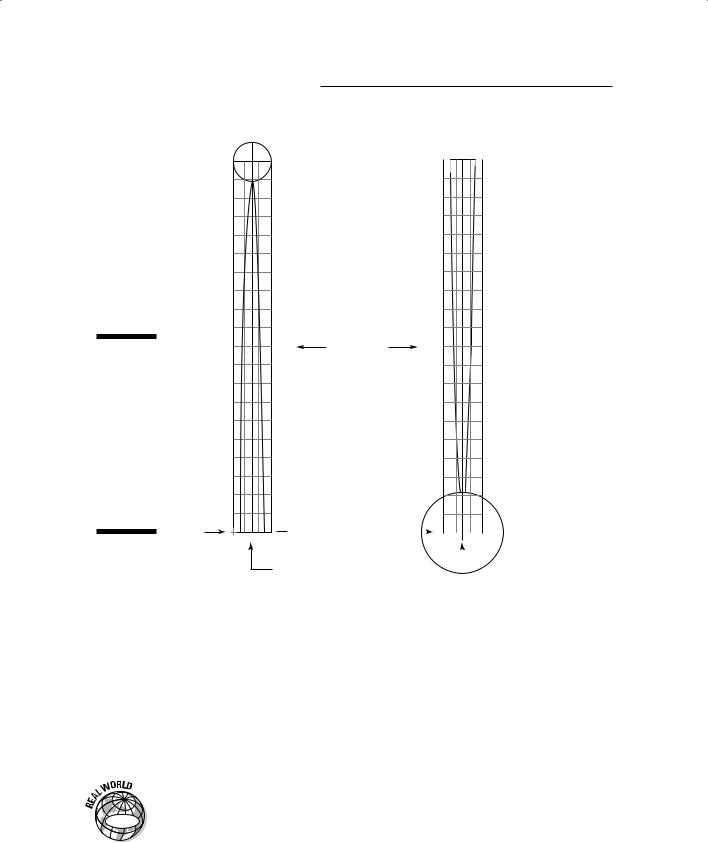
Figure 2-5 shows a diagram of the UTM coordinate system. The zones are numbered, starting at the 180th meridian, in an eastward direction. Each zone is divided into rows (or sections) of 8 degrees latitude each, with the exception of the northernmost section, which is 12 degrees, allowing the system to cover all the land of the northern hemisphere. You can isolate small sections of the Earth because you locate them by a number/letter combination. With the exception of the northernmost group, each of these sections occupies 100,000 meters on a side and can be designated by eastings and northings (that is, positive measurements eastward and northward of the origin) of up to five-digit accuracy (1-meter level resolution).
36 |
Part I: GIS: Geography on Steroids |
North Zone |
South Zone |
Figure 2-5:
The UTM coordinate system showing origins, zones, sections, and the numbering and lettering system.
N Origin
0 E, 0 N
10,000,000 

 Equator
meters N
5,000,000 meters N
Equator |
S Origin |
|
|
|
|
|
|
|
|
|
500,000 |
0 E, 0 N |
|
|
500,000 |
||||||
|
||||||||||
|
|
|
|
|
|
|
|
|||
|
|
|
|
|
|
|
|
|||
meters E |
|
|
|
|
|
|
|
|
meters E |
|
Measuring the land
Coordinate systems help you measure geographic features, as well as find your way around and locate things on a map. One major feature you’ll likely encounter in your GIS work is land ownership, and you’ll find many systems that measure and record this feature. I describe a common one used in the United States to help you understand the relationship between land measurement and the coordinate system.
|
The U.S. Public Land Survey System (PLSS) was established in the late 1700s |
|
|
to divide up the ever increasing lands that the U.S. Government acquired. The |
|
GIS |
PLSS is similar to a rectangular coordinate system, but it’s not directly linked |
|
to any particular map projection. |
||
|

Chapter 2: Recognizing How Maps Show Information 37
Maps as questions, as well as answers
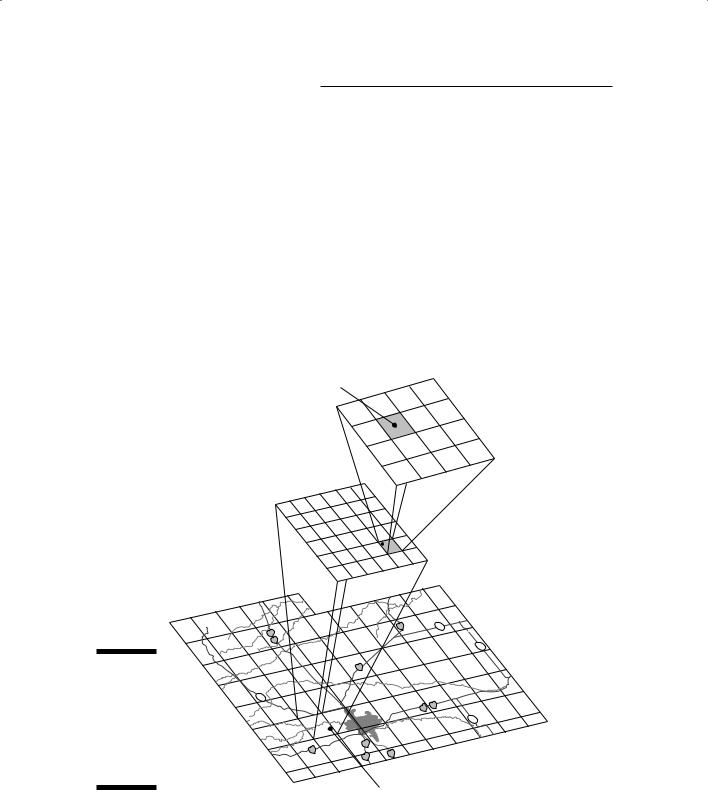
Most map readers assume the map is accurate, which isn’t always true, depending on the scale. More importantly, though, most believe that the map answers the question, “Where is ______?” You fill in the blank. Well, I’m not going to argue with you there — the map really does display (within its graphic and scale limits) locations and distributions of all sorts of geographic features. But that’s just the beginning. The geographer and the GIS professional often see a map as just the beginning, rather than an end.
Let me help you understand where these folks are coming from. The GIS is designed to input data from maps, and then compare the locations and distributions of geographic features from one map to another. Well, would you add map data into the GIS if you didn’t think that you could use the data for analysis? And you probably select your maps with particular questions in mind. Because you’re using maps, it’s also a safe bet that your questions revolve around the locations and patterns of the geographic features you choose to include.
So, for example, if you’re a crime analyst, you might have a map of auto thefts for your city. This map answers the question, “Where are the auto thefts?” But, if you needed to know only where thefts occur, you wouldn’t need to put it into the computer. You have questions about the locations and distributions. You might want to know some of the following:
Do the auto thefts occur more in some areas than in others — does your city have auto theft “hot spots”?
Do the number of cars stolen increase at any particular time of day, day of the week, month, or year (is there a temporal pattern)?
Do other distributions seem to match that of the auto thefts? Or, stated differently, do spatial correlations exist between auto thefts and other factors, such as neighborhood type, access to major highways, or gang activity?
The map is both an answer and a question. When you look at a map, especially if you’re considering including it in a GIS database, you should start asking questions about the distributions and patterns that you observe. The question is always the same — “What explains this distribution?” GIS gives you tools to answer that question. And if you can explain a distribution, you can begin to predict future distributions and make plans accordingly.
So, if you’re a transportation planner and you notice that the traffic counts are increasing in a particular neighborhood, your analysis might show that this traffic increase is very strongly related to population increases in certain neighborhoods. Your next step might be to build a predictive map of future transportation while the population grows. You can then use that prediction to suggest improvements to the transportation system. In a way, GIS makes you a really great prognosticator.
This land ownership recording system is based on the acre, which is 1/640 of a square mile (a section). Thirty-six sections are grouped together into townships and numbered in serpentine fashion from upper-right (section 1) to lower-right (section 36). A land records specialist can subdivide these chunks of land into halves and quarters so that he or she can describe the land holdings by these fractions. For example, the PLSS system describes the plot of land you own as something like NE1/4 SE1/4 N1/2 Sect. 23, T144, R35E.
38 |
Part I: GIS: Geography on Steroids |
Figure 2-6:
Subdividing land by using the PLSS, or township and range, system.
All these land portions are part of a larger coordinate system of horizontal and vertical lines. Distance is measured north and south (township) of starting lines called baselines, and east and west (range) from starting lines
called principal meridians. These township and range lines allow for the legal descriptions of land.
The notation that identifies a parcel of land starts with the smallest subdivision of land, then gives the section number, and then township and range numbers. A legal land description based on this system includes the state name, principal meridian name, township and range designations, and section number. Figure 2-6 shows a breakdown of the PLSS system.
Such land subdivision systems enable you to build GIS databases that have land ownership correlated to other factors, such as zoning restrictions or price per acre.
Well name Bailey No. 1
Location SE NW Sec. 26 T14N R68W
|
|
|
|
|
|
|
|
|
|
|
|
NW |
|
|
NE |
|
|
NE |
|||||
|
|
|
|
|
|
|
|
|
|
|
|
NW |
|
|
|
|
|
|
|||||
|
|
|
|
|
|
|
|
|
|
|
|
|
|
|
|
|
|
|
|
|
|||
|
|
|
|
|
|
|
|
|
|
|
|
|
|
|
SW |
|
|
|
|
.28 |
|||
|
|
|
|
|
|
|
|
|
|
|
|
|
|
|
|
|
Sec |
|
|||||
|
|
|
|
|
|
|
|
|
|
|
|
|
|
|
|
|
|
|
|
SW |
|
|
|
|
|
|
|
|
|
. |
|
|
|
|
|
|
|
|
|
|
|
|
|
|
|
|
|
|
|
|
|
|
W |
|
|
|
|
|
|
|
|
|
|
|
|
|
|
|
|
|
|
|
|
|
|
.68 |
|
|
|
|
|
|
|
|
1 |
|
|
|
|
|
|
|
|
||
|
|
|
R |
|
|
3 |
|
|
2 |
|
|
|
|
|
|
|
|
|
|||||
|
|
|
|
|
4 |
|
|
|
|
|
|
|
|
|
|
|
|
|
|
||||
|
|
|
5 |
|
|
|
|
|
|
|
|
|
12 |
|
|
|
|
|
|
||||
|
6 |
|
|
|
|
|
|
|
|
|
|
11 |
|
|
|
|
|
|
|
||||
|
|
|
|
|
|
|
|
10 |
|
|
|
|
|
|
|
|
|
||||||
|
|
|
|
|
9 |
|
|
|
|
|
|
13 |
|
|
|
. |
|||||||
|
|
|
|
8 |
|
|
|
|
|
|
|
|
|
|
|||||||||
|
|
|
|
|
|
|
|
|
|
|
|
|
|
|
|
||||||||
|
|
|
|
|
|
|
|
|
|
|
|
|
|
|
|
|
N |
||||||
|
|
7 |
|
|
|
|
|
|
|
|
|
|
|
|
14 |
|
|
|
.14 |
|
|||
|
|
|
|
|
|
16 |
|
15 |
|
|
|
T |
|
|
|
||||||||
|
|
|
|
|
17 |
|
|
|
|
|
24 |
|
|
|
|||||||||
|
|
|
18 |
|
|
|
|
|
|
23 |
|
|
|
||||||||||
|
|
|
|
|
|
|
|
|
|
22 |
|
|
|
|
|||||||||
|
|
|
|
|
|
|
|
|
21 |
|
|
|
|
|
|
||||||||
|
|
|
|
|
|
|
20 |
|
|
|
|
|
25 |
|
|
|
|||||||
|
|
|
|
|
19 |
|
|
|
|
|
|
|
26 |
|
|
|
|||||||
|
|
|
|
|
|
|
|
|
|
|
|
27 |
|
|
|
|
|||||||
|
|
|
|
|
|
|
|
|
|
|
|
|
|
|
|
|
|||||||
|
|
|
|
|
|
|
|
|
|
|
|
|
28 |
|
|
|
36 |
|
|||||
|
|
|
|
|
|
|
|
|
|
29 |
|
|
|
|
|
|
|
||||||
|
|
|
|
|
|
30 |
|
|
|
|
|
|
|
34 |
35 |
|
|||||||
|
|
|
|
|
|
|
|
|
|
|
|
|
|
|
|
|
|||||||
|
|
|
|
|
|
|
|
|
|
|
|
|
33 |
|
|
|
|
||||||
|
|
|
|
|
|
|
|
|
|
|
32 |
|
|
|
|
|
|||||||
|
|
|
|
|
|
|
|
|
31 |
|
|
|
|
|
|
|
|
|
|||||
|
|
|
|
|
|
|
|
|
|
|
|
|
|
|
|
|
|
|
|
||||
|
|
|
|
|
|
|
|
|
|
|
|
|
|
|
|
|
|
|
|
|
|
||
|
104˚45 |
|
|
|
19 |
N. |
|
|
|
|
|
|
|
|
|
|
|
104˚15 |
|
|
|
||
|
|
|
|
|
|
|
|
|
|
|
|
|
|
|
|
|
|
|
|
||||
|
|
|
|
|
|
|
|
|
|
|
|
|
|
|
|
|
|
|
|
|
|||
105˚00 |
|
|
|
T. |
|
|
104˚30 |
|
|
|
|
|
|
|
|
|
|||||||
|
|
|
|
|
|
|
|
|
|
|
|
|
|
|
|
||||||||
105˚15
SE
|
N. |
|
|
T. |
18 |
|
|
|
|
|
|
|
|
N. |
|
|
T. |
17 |
|
|
|
|
|
|
|
|
N. |
|
|
T. |
16 |
|
|
|
41˚30
41˚15
41˚00
|
|
|
|
|
|
|
|
|
|
|
|
County |
|
|
|
|
|
|
|
.15 |
N. |
|
|
|
|
|
||
|
|
|
|
|
|
|
|
|
Laramie |
|
|
|
|
|
|
|
T |
|
|
|
|
|
|
|||||
|
|
|
|
|
|
|
|
|
|
|
|
|
|
|
|
|
|
|
|
|
|
N. |
|
|
|
|||
|
|
|
|
|
|
|
|
|
|
|
|
|
|
|
|
|
|
|
|
|
|
|
|
|
|
|
|
|
|
|
|
|
|
|
|
|
|
|
|
|
|
|
|
|
|
|
|
|
|
|
|
T. |
14 |
|
|
|
|
|
|
|
|
|
|
|
|
|
|
|
|
|
|
|
|
|
|
|
Bluffs |
|
|
|
|
|
|
|
||
|
|
|
|
|
|
|
|
|
|
|
|
|
|
|
|
|
Pine |
|
|
|
|
|
|
N. |
||||
|
|
|
|
|
|
|
|
|
|
|
|
|
|
|
|
|
|
|
|
|
|
|
|
|
||||
|
|
|
|
|
|
|
|
|
|
|
|
|
|
|
|
|
|
|
|
|
|
|
|
|
|
|
||
|
|
|
|
|
|
|
|
|
|
|
|
|
|
|
|
|
|
|
|
|
|
|
|
|
T. |
13 |
|
|
|
|
|
|
|
|
|
|
|
|
|
|
|
|
|
|
|
|
|
|
|
|
|
|
|
|
|
|
|
|
|
|
|
|
|
|
|
|
|
|
|
|
|
|
|
|
|
|
|
|
|
|
|
|
|
|
|
N. |
|
|
|
|
|
|
|
|
|
|
|
|
|
|
|
|
|
|
|
|
|
|
|
|
|
|
|
T. |
12 |
|
|
|
|
|
|
|
|
|
|
|
|
|
|
|
|
|
|
|
|
|
|
|
|
|
|
|
|
|
|
|
|
|
|
|
Cheyenne |
|
|
|
|
|
|
|
|
|
|
|
|
|
|
|
|
|
|
. |
|||
|
|
|
|
|
|
|
|
|
|
|
|
|
|
|
|
|
|
|
|
|
|
|
|
|
.R. |
60 |
W |
|
|
|
|
|
|
|
|
|
|
|
|
|
|
|
|
|
|
|
|
|
|
|
|
|
|
|
|||
|
|
|
|
|
|
|
|
|
|
|
|
|
|
Carpenter |
|
|
|
|
|
|
.61 |
W |
|
|
|
|||
|
|
|
|
|
|
|
|
|
|
|
|
|
|
|
|
|
|
|
|
|
|
.R |
|
|
|
|
|
|
|
|
|
|
|
|
|
|
|
|
|
|
|
|
|
|
|
|
|
|
.62 |
W |
|
|
|
|
|
|
|
|
|
|
|
|
|
|
|
|
|
|
|
|
|
|
|
|
|
|
.R |
|
|
|
|
|
|
|
|
|
|
|
|
|
|
|
|
|
|
|
|
|
|
|
|
|
|
|
W |
|
|
|
|
|
|
|
|
|
|
|
|
|
|
|
|
|
|
|
|
|
|
|
|
|
|
|
.63 |
|
|
|
|
|
|
|
|
|
|
|
|
|
|
|
|
|
|
|
|
|
|
|
|
|
|
|
.R |
|
|
|
|
|
|
|
|
|
|
|
|
|
|
|
|
|
|
|
|
|
|
|
|
|
|
|
.64 |
W |
|
|
|
|
|
|
|
|
|
|
|
|
|
|
|
|
|
|
|
|
|
|
|
|
|
|
.R |
|
|
|
|
|
|
|
|
|
|
|
|
|
|
|
|
|
|
|
|
|
|
|
|
|
|
|
.65 |
W |
|
|
|
|
|
|
|
|
|
|
|
|
|
|
|
|
|
|
|
|
|
|
|
|
|
|
.R |
|
|
|
|
|
|
|
|
|
|
|
|
|
|
|
|
|
|
|
|
|
|
|
|
|
|
|
W |
|
|
|
|
|
|
|
|
|
|
|
|
|
|
|
|
|
|
|
|
|
|
|
|
|
|
|
.66 |
|
|
|
|
|
|
|
|
|
|
|
|
|
|
|
|
|
|
|
|
|
|
|
|
|
|
|
.R |
|
|
|
|
|
|
|
|
|
|
|
|
|
|
|
|
|
|
|
|
|
|
|
|
|
|
|
.67 |
W |
|
|
|
|
|
|
|
|
|
|
|
|
|
|
|
|
|
|
|
|
|
|
|
|
|
|
.R |
|
|
|
|
|
|
|
|
|
|
|
|
|
|
|
|
|
|
|
|
|
|
|
|
|
|
.68 |
W |
|
|
|
|
|
|
|
|
|
|
|
|
|
|
|
|
|
|
|
|
|
|
|
|
|
|
.R |
|
|
|
|
|
|
|
|
|
|
|
|
|
|
|
|
|
|
|
|
|
|
|
|
|
|
|
.69 |
W |
|
|
|
|
|
|
|
|
|
|
|
|
|
|
|
|
|
|
|
|
|
|
|
|
|
|
.R |
|
|
|
|
|
|
|
|
|
|
|
|
|
|
|
|
|
|
|
|
|
|
|
|
|
|
R. |
70 |
W |
|
|
|
|
|
|
Well name Bailey No. 1 |
|
|
|
|
|
|
|
|
|
||||||||||
|
|
|
|
|
|
|
|
|
|
|
|
|
|
|
|
|
|
|
|
|
|
|
|
|
|
|
||
|
|
|
|
|
|
|
|
|
|
|
|
|
|
|
|
|
|
|
|
|
|
|
|
|
|
|
|
|
Location SE NW Sec. 26 T14N R68W

Chapter 3
Reading, Analyzing, and
Interpreting Maps
In This Chapter
Translating map symbols
Spotting patterns
Analyzing the patterns you identify
Applying your conclusions to the decision-making process
People who explore GIS are often most astonished by the wide variety of content-specific (thematic) maps available. You need to have a working
knowledge of the many varieties of maps and the types of symbols they use so that you can determine the best way to input data, as well as know the types of maps you use for a given application.
While you become familiar with maps, especially thematic maps, you begin to identify patterns in the symbols on the paper. Spotting patterns isn’t as easy as you might think because those abstract symbols represent sensory data contained on the map. The experience is akin to finding your way around a new town — you get the hang of it while you press further into your exploration.
This chapter shows you how to identify patterns within the sometimes complex map symbology. Also, you can find out how to ask questions about the patterns you identify, answer those questions through GIS analysis, and ultimately make decisions based on your analysis.

40 |
Part I: GIS: Geography on Steroids |
Making Sense of Symbols
Many types of maps are available, and each type has a unique set of symbols. Symbols are lines, objects, or pictures on the map that represent real objects on the ground. With so many map types, each with its own set of symbols, you can easily become confused when trying to interpret the maps. You can make the process easier on yourself by looking at the dimensions and the types of measurement scales available for mapping and GIS operations, as described in the following sections.
Categorizing the space on a map
Categorizing the space represented on maps helps make symbology easier to understand. The types of space that occur in maps are
Points: Considered zero-dimensional because they take up no space at all. Points show up as symbols representing the locations of objects such as towns, wells, or churches. These symbols might be dots for towns, a tiny caricature of a well for wells, or a cross for Christian churches.
Lines: One-dimensional (measured by length). Lines might be streets, roads, or railroad tracks symbolized by different types or colors of lines on the map.
Areas: Two-dimensional (measured by length and width). Areas might be color patterns on city street maps that indicate different neighborhoods or suburbs, or they might be patches of blue to show the location of lakes.
Volumes: Three-dimensional (measured by length, width, and depth or height).Volume spaces are important when you want to identify something such as a buried coal seam. Volumes show up as area symbols on a map.
When it comes to map symbols, volumes and surfaces are treated pretty much the same. Unlike volumes, however, surfaces are thought to “blanket” something, rather than include what’s inside. For example, if you’re interested in the vegetation covering a mountain, you’re really interested in only the elevation’s surface. But, if you’re interested in how much coal is located underground, you need to know not just the surface of the ore seam, but also its whole volume because you’ll be extracting that volume.
Four types of objects are symbolized on your map — points (zerodimensional), lines (one-dimensional), areas (two-dimensional), and volumes (three-dimensional).