

- •Preface
- •Acknowledgements
- •Contents
- •1.1 Introduction
- •1.2 Classical Physics Between the End of the XIX and the Dawn of the XX Century
- •1.2.1 Maxwell Equations
- •1.2.2 Luminiferous Aether and the Michelson Morley Experiment
- •1.2.3 Maxwell Equations and Lorentz Transformations
- •1.3 The Principle of Special Relativity
- •1.3.1 Minkowski Space
- •1.4 Mathematical Definition of the Lorentz Group
- •1.4.1 The Lorentz Lie Algebra and Its Generators
- •1.4.2 Retrieving Special Lorentz Transformations
- •1.5 Representations of the Lorentz Group
- •1.5.1 The Fundamental Spinor Representation
- •1.6 Lorentz Covariant Field Theories and the Little Group
- •1.8 Criticism of Special Relativity: Opening the Road to General Relativity
- •References
- •2.1 Introduction
- •2.2 Differentiable Manifolds
- •2.2.1 Homeomorphisms and the Definition of Manifolds
- •2.2.2 Functions on Manifolds
- •2.2.3 Germs of Smooth Functions
- •2.3 Tangent and Cotangent Spaces
- •2.4 Fibre Bundles
- •2.5 Tangent and Cotangent Bundles
- •2.5.1 Sections of a Bundle
- •2.5.2 The Lie Algebra of Vector Fields
- •2.5.3 The Cotangent Bundle and Differential Forms
- •2.5.4 Differential k-Forms
- •2.5.4.1 Exterior Forms
- •2.5.4.2 Exterior Differential Forms
- •2.6 Homotopy, Homology and Cohomology
- •2.6.1 Homotopy
- •2.6.2 Homology
- •2.6.3 Homology and Cohomology Groups: General Construction
- •2.6.4 Relation Between Homotopy and Homology
- •References
- •3.1 Introduction
- •3.2 A Historical Outline
- •3.2.1 Gauss Introduces Intrinsic Geometry and Curvilinear Coordinates
- •3.2.3 Parallel Transport and Connections
- •3.2.4 The Metric Connection and Tensor Calculus from Christoffel to Einstein, via Ricci and Levi Civita
- •3.2.5 Mobiles Frames from Frenet and Serret to Cartan
- •3.3 Connections on Principal Bundles: The Mathematical Definition
- •3.3.1 Mathematical Preliminaries on Lie Groups
- •3.3.1.1 Left-/Right-Invariant Vector Fields
- •3.3.1.2 Maurer-Cartan Forms on Lie Group Manifolds
- •3.3.1.3 Maurer Cartan Equations
- •3.3.2 Ehresmann Connections on a Principle Fibre Bundle
- •3.3.2.1 The Connection One-Form
- •Gauge Transformations
- •Horizontal Vector Fields and Covariant Derivatives
- •3.4 Connections on a Vector Bundle
- •3.5 An Illustrative Example of Fibre-Bundle and Connection
- •3.5.1 The Magnetic Monopole and the Hopf Fibration of S3
- •The U(1)-Connection of the Dirac Magnetic Monopole
- •3.6.1 Signatures
- •3.7 The Levi Civita Connection
- •3.7.1 Affine Connections
- •3.7.2 Curvature and Torsion of an Affine Connection
- •Torsion and Torsionless Connections
- •The Levi Civita Metric Connection
- •3.8 Geodesics
- •3.9 Geodesics in Lorentzian and Riemannian Manifolds: Two Simple Examples
- •3.9.1 The Lorentzian Example of dS2
- •3.9.1.1 Null Geodesics
- •3.9.1.2 Time-Like Geodesics
- •3.9.1.3 Space-Like Geodesics
- •References
- •4.1 Introduction
- •4.2 Keplerian Motions in Newtonian Mechanics
- •4.3 The Orbit Equations of a Massive Particle in Schwarzschild Geometry
- •4.3.1 Extrema of the Effective Potential and Circular Orbits
- •Minimum and Maximum
- •Energy of a Particle in a Circular Orbit
- •4.4 The Periastron Advance of Planets or Stars
- •4.4.1 Perturbative Treatment of the Periastron Advance
- •References
- •5.1 Introduction
- •5.2 Locally Inertial Frames and the Vielbein Formalism
- •5.2.1 The Vielbein
- •5.2.2 The Spin-Connection
- •5.2.3 The Poincaré Bundle
- •5.3 The Structure of Classical Electrodynamics and Yang-Mills Theories
- •5.3.1 Hodge Duality
- •5.3.2 Geometrical Rewriting of the Gauge Action
- •5.3.3 Yang-Mills Theory in Vielbein Formalism
- •5.4 Soldering of the Lorentz Bundle to the Tangent Bundle
- •5.4.1 Gravitational Coupling of Spinorial Fields
- •5.5 Einstein Field Equations
- •5.6 The Action of Gravity
- •5.6.1 Torsion Equation
- •5.6.1.1 Torsionful Connections
- •The Torsion of Dirac Fields
- •Dilaton Torsion
- •5.6.2 The Einstein Equation
- •5.6.4 Examples of Stress-Energy-Tensors
- •The Stress-Energy Tensor of the Yang-Mills Field
- •The Stress-Energy Tensor of a Scalar Field
- •5.7 Weak Field Limit of Einstein Equations
- •5.7.1 Gauge Fixing
- •5.7.2 The Spin of the Graviton
- •5.8 The Bottom-Up Approach, or Gravity à la Feynmann
- •5.9 Retrieving the Schwarzschild Metric from Einstein Equations
- •References
- •6.1 Introduction and Historical Outline
- •6.2 The Stress Energy Tensor of a Perfect Fluid
- •6.3 Interior Solutions and the Stellar Equilibrium Equation
- •6.3.1 Integration of the Pressure Equation in the Case of Uniform Density
- •6.3.1.1 Solution in the Newtonian Case
- •6.3.1.2 Integration of the Relativistic Pressure Equation
- •6.3.2 The Central Pressure of a Relativistic Star
- •6.4 The Chandrasekhar Mass-Limit
- •6.4.1.1 Idealized Models of White Dwarfs and Neutron Stars
- •White Dwarfs
- •Neutron Stars
- •6.4.2 The Equilibrium Equation
- •6.4.3 Polytropes and the Chandrasekhar Mass
- •6.5 Conclusive Remarks on Stellar Equilibrium
- •References
- •7.1 Introduction
- •7.1.1 The Idea of GW Detectors
- •7.1.2 The Arecibo Radio Telescope
- •7.1.2.1 Discovery of the Crab Pulsar
- •7.1.2.2 The 1974 Discovery of the Binary System PSR1913+16
- •7.1.3 The Coalescence of Binaries and the Interferometer Detectors
- •7.2 Green Functions
- •7.2.1 The Laplace Operator and Potential Theory
- •7.2.2 The Relativistic Propagators
- •7.2.2.1 The Retarded Potential
- •7.3 Emission of Gravitational Waves
- •7.3.1 The Stress Energy 3-Form of the Gravitational Field
- •7.3.2 Energy and Momentum of a Plane Gravitational Wave
- •7.3.2.1 Calculation of the Spin Connection
- •7.3.3 Multipolar Expansion of the Perturbation
- •7.3.3.1 Multipolar Expansion
- •7.3.4 Energy Loss by Quadrupole Radiation
- •7.3.4.1 Integration on Solid Angles
- •7.4 Quadruple Radiation from the Binary Pulsar System
- •7.4.1 Keplerian Parameters of a Binary Star System
- •7.4.2 Shrinking of the Orbit and Gravitational Waves
- •7.4.2.1 Calculation of the Moment of Inertia Tensor
- •7.4.3 The Fate of the Binary System
- •7.4.4 The Double Pulsar
- •7.5 Conclusive Remarks on Gravitational Waves
- •References
- •Appendix A: Spinors and Gamma Matrix Algebra
- •A.2 The Clifford Algebra
- •A.2.1 Even Dimensions
- •A.2.2 Odd Dimensions
- •A.3 The Charge Conjugation Matrix
- •A.4 Majorana, Weyl and Majorana-Weyl Spinors
- •Appendix B: Mathematica Packages
- •B.1 Periastropack
- •Programme
- •Main Programme Periastro
- •Subroutine Perihelkep
- •Subroutine Perihelgr
- •Examples
- •B.2 Metrigravpack
- •Metric Gravity
- •Routines: Metrigrav
- •Mainmetric
- •Metricresume
- •Routine Metrigrav
- •Calculation of the Ricci Tensor of the Reissner Nordstrom Metric Using Metrigrav
- •Index

7.4 Quadruple Radiation from the Binary Pulsar System |
301 |
Let us make a numerical comparison between the binary system case and the perihelion advance of mercury where:
|
Δϕ |
|
3 |
[GMS ]3/2 |
1 |
(7.4.13) |
|
|
aM5/2(1 − eM2 ) |
||||
|
T |
Merc = |
|
c2 |
|
MS being the solar mass and aM , eM the geometrical parameters of Mercury orbit, while aBS, eBS are those of the binary star system.
Defining the dimensionless factors:
|
|
|
x |
= |
|
(μ1 + μ2) |
|
|
|
(7.4.14) |
|||
|
|
|
|
|
|
|
|||||||
|
|
|
|
|
|
MS |
|
|
|
|
|
||
|
|
|
y = |
aM |
|
|
|
|
(7.4.15) |
||||
|
|
|
aBS |
|
|
|
|
|
|||||
|
|
|
z |
= |
|
1 − eM2 |
|
|
(7.4.16) |
||||
|
|
|
1 − eBS2 |
||||||||||
|
|
|
|
|
|
|
|
|
|
|
|||
we obtain the relation |
|
|
|
|
|
|
|
|
|
|
|
||
|
Δϕ |
|
BS = |
y5/2x3/2z |
Δϕ |
|
(7.4.17) |
||||||
|
|
||||||||||||
|
T |
|
|
|
|
|
|
T Merc |
|
||||
Numerically we have: |
|
|
|
|
|
|
|
|
|
|
|
||
z = 1.547 |
|
y = 28.46 |
|
|
x = 2.8275 |
(7.4.18) |
|||||||
and hence the factor |
|
|
|
|
|
|
|
|
|
|
|
||
|
f = y5/2x3/2z 31782 |
(7.4.19) |
|||||||||||
While for mercury the angular advance is |
|
|
|
|
|
||||||||
|
|
|
|
42 /century |
|
|
|
|
(7.4.20) |
||||
for the pulsar binary system we get: |
|
|
|
|
|
|
|
|
|
||||
|
|
Δϕ 3.7 deg/year |
(7.4.21) |
||||||||||
As we see the overwhelming contribution to this enhancement is due to the narrowness of the system, namely the ratio between the semilati recti.
7.4.2 Shrinking of the Orbit and Gravitational Waves
We have indirect evidence of the emission of gravitational waves from the decrease of the period T and the consequent shrinking of the orbit, namely the decrease of the semilatus rectum. From (7.4.6), by taking a time derivative, we obtain
302 |
7 Gravitational Waves and the Binary Pulsars |
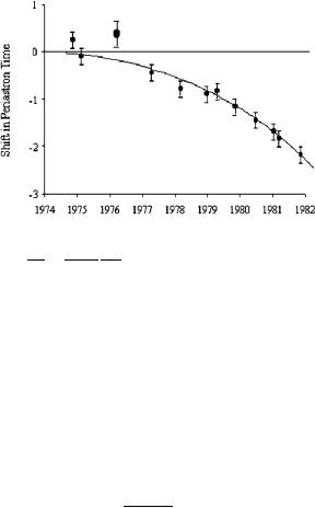
Fig. 7.14 The decrease in the period and the shrinking of the orbit for the pulsar binary system PRS1913+16
da = μ1μ2 dE
dt 2E2 dt
(7.4.22)
so that a shrinking of the orbit, corresponds to a decrease of the system energy. Such energy is radiated away in the form of gravitational waves. It is extremely interesting to perform an accurate calculation of such of energy loss by quadrupole radiation in order to compare with experimental data on the reduction of the period (see Fig. 7.14).
7.4.2.1 Calculation of the Moment of Inertia Tensor
We consider Fig. 7.15 and calling r the vector joining one of the two stars with the other we can write:
r1 = |
μ2 |
|
μ1 |
|
|
|
r; |
r2 = |
μ1 + μ2 r |
(7.4.23) |
|
μ1 + μ2 |
|||||
where, according to Kepler laws and the Newtonian solution of the dynamical problem we have:
r r |
|
a(1 − e2) |
(7.4.24) |
||
|
|
||||
≡ | | = |
1 |
+ |
e cos θ |
|
|
|
|
||||
Then we define the moment of inertia according to:
Ik |
≡ |
|
ρ(x)xk x |
= |
μ1rk |
, r |
+ |
μ2rk |
, r |
||
|
|
|
|
|
1 |
1 |
2 |
2 |
|||
|
|
|
|
μ1μ2 |
|
|
|
|
|
|
|
|
= |
|
|
rk r |
|
|
|
|
|
(7.4.25) |
|
|
|
μ1 + μ2 |
|
|
|
|
|
||||
Then turning to polar coordinates:
r1 ≡ x = r cos θ ; r2 ≡ y = r sin θ ; r3 ≡ z = 0 |
(7.4.26) |

7.4 Quadruple Radiation from the Binary Pulsar System |
303 |
Fig. 7.15 The vectors defining the position of the two stars with respect to their center of mass
we obtain:
Ixx = |
μ1μ2 |
2 cos2 θ |
|
|
r |
||
μ1 + μ2 |
|||
Iyy = |
μ1μ2 |
2 sin2 θ |
|
|
r |
||
μ1 + μ2 |
|||
Ixy = |
μ1μ2 |
2 sin θ cos θ |
|
|
r |
||
μ1 + μ2 |
|||
TrI = |
μ1μ2 |
2 |
|
|
r |
||
μ1 + μ2 |
|
||
The angular momentum, on the other hand is:
= |
|
μ1μ2 |
|
2θ |
|
μ1 + μ2 r |
|||||
˙ |
|||||
(7.4.27)
(7.4.28)
Recalling the relation between the angular momentum , the energy E and the geometrical parameters of the orbit a and e, displayed in (7.4.6) by comparison with (7.4.28), we obtain:
|
|
1 |
|
|
|
|
|
|
|
|
|
|
θ |
|
(μ1 |
+ |
μ2) 1 |
− |
e2 |
aG |
|||||
|
|
|||||||||||
˙ = r2 |
|
|
|
|
|
|
||||||
|
|
|
|
|
|
|
|
|
|
|
(7.4.29) |
|
r |
e sin θ |
9 |
|
μ1 + μ2 |
G |
|
|
|
||||
|
|
|
|
|
||||||||
˙ = |
|
|
|
|
|
|
a(1 − e2) |
|
|
|
||
This information suffices to calculate the third derivative of the inertia tensor which, turning to natural units where G = c = 1, takes the following form:
d3Ixx |
= |
2 |
|
|
μ1μ2 |
|
2 sin 2θ |
+ |
3e cos2 |
|
|
θ |
|
|
|
|||||
dt3 |
a(1 − e2) |
|
|
|
|
|
||||||||||||||
|
|
|
|
|
|
θ sin θ ˙ |
|
|
|
|||||||||||
d3Iyy |
= − |
2 |
μ1μ2 |
|
2 sin 2θ |
+ |
3e cos2 |
θ sin θ |
|
θ |
|
|||||||||
|
|
|
− e2) |
|
|
|||||||||||||||
dt3 |
|
a(1 |
|
|
|
|
|
|
|
+ e sin θ ˙ |
(7.4.30) |
|||||||||
d3Ixy |
= − |
2 |
μ1μ2 |
|
2 cos 2θ |
− |
e cos θ |
+ |
3e cos3 |
θ |
|
|||||||||
dt3 |
a(1 − e2) |
|
||||||||||||||||||
|
|
|
|
|
|
|
|
θ ˙ |
|
|||||||||||
|
d3I |
|
|
|
|
μ1μ2 |
|
e sin |
θ |
|
|
|
|
|
|
|
|
|||
|
dt3 |
= −2 a(1 |
|
e2) |
|
|
|
|
|
|
|
|
||||||||
|
− |
|
θ |
˙ |
|
|
|
|
|
|
|
|
||||||||
|
|
|
|
|
|
|
|
|
|
|
|
|
|
|
|
|
|
|
|
|

304 7 Gravitational Waves and the Binary Pulsars
The quadrupole moment Qij is related to moment of inertia by a very simple relation:
|
= |
|
− |
3 |
|
|
|
Qij |
|
3 Iij |
|
1 |
δij I |
|
(7.4.31) |
|
|
|
so that by means of the above results we can immediately calculate its third derivative. The relevant squared modulus appearing in the Einstein formula (7.3.94) is then easily obtained:
... ... |
|
1 |
... |
|
... ... |
|
1 |
... |
|
|
||||||
Q |
Qij |
= |
I |
2 |
+ |
2 I |
2 |
+ |
I |
2 |
− |
I 2 |
|
(7.4.32) |
||
9 |
|
|
|
3 |
||||||||||||
ij |
|
|
xx |
|
xy |
|
yy |
|
|
|
||||||
and in natural units G = c = 1, we obtain:
|
dE |
|
1 |
... |
|
2 |
2 |
|
|
|
|
|
|
|
|
|
|
|
= |
Q |
2 |
8μ1 |
μ2 |
|
12(1 |
+ |
e cos θ )2 |
|
2 |
2 |
θ |
2 |
|
||
− dt |
45 |
ij | = |
15a2(1 − e2)2 |
|
+ e |
|
sin |
|
(7.4.33) |
||||||||
| |
|
|
|
θ ˙ |
|
||||||||||||
We can average the energy loss over one revolution period defining:
> dE ? |
= − |
1 2π dE dθ |
||||||
− |
|
|
|
|
|
|
|
|
dt |
T |
0 |
dt θ |
|||||
|
|
|
|
|
|
|
˙ |
|
With straightforward algebra we obtain:
|
1 dE |
= |
|
8μ12μ22 |
|
|
|
|
+ |
e cos θ ) |
2 |
+ |
2 |
2 |
˙ |
||||
|
|
|
|
|
|
|
|
|
e |
|
|||||||||
θ dt |
|
15a2(1 e2)2 |
|
|
|
||||||||||||||
|
˙ |
|
|
− |
|
12(1 |
|
|
|
|
sin θ θ |
||||||||
|
|
|
|
|
|
|
|
|
|
|
|
|
|
|
|
||||
|
|
|
|
|
|
32μ12μ22 |
|
√ |
|
|
|
|
|
where |
|
||||
|
|
|
|
= |
|
|
μ1 |
+ |
μ2f (θ, e) |
|
|||||||||
|
|
|
|
|
|
7 |
|
||||||||||||
|
|
|
|
|
5(a(1 − e2)) 2 |
|
|
|
|
|
|
1 |
|
|
|
||||
f (θ, e) ≡ |
(1 + e cos θ )2 (1 + e cos θ )2 + |
|
|
|
|
||||||||||||||
12 e2 sin2 θ |
|||||||||||||||||||
(7.4.34)
(7.4.35)
Using Kepler third law we can express the period of revolution in terms of the semilatus rectum:
3
T = √ 2π a 2 (7.4.36)
μ1 + μ2
which, inserted in (7.4.34), yields
> |
dE |
? |
= |
32 |
|
μ12μ22 |
|
(μ1 |
+ |
μ2) |
1 |
|
1 |
2π f (θ, e) |
(7.4.37) |
|
|
5 |
|
|
|
|
a5 2π |
||||||||||
− dt |
1 |
− e2 |
7 |
|
|
0 |
|
|||||||||
|
|
|
|
|
2 |
|
|
|
|
|
|
|
||||
The integral appearing in (7.4.37) is easily evaluated and one obtains the following final expression for the average energy loss during each revolution (still written in natural units G = c = 1):

7.4 Quadruple Radiation from the Binary Pulsar System |
305 |
>?
− |
dE |
= |
32 1 |
μ12μ22(μ1 |
+ μ2)f(e) |
(7.4.38) |
||||||||||||
|
dt |
5 |
|
a5 |
||||||||||||||
|
|
|
|
T |
|
|
|
|
|
|
|
|
|
|
|
|
|
|
where: |
|
|
|
|
|
|
|
|
|
|
|
|
|
|
|
|
|
|
f(e) |
≡ |
|
1 |
|
1 |
+ |
|
73 |
e2 |
+ |
37 |
e4 |
|
(7.4.39) |
||||
|
|
1 |
24 |
96 |
||||||||||||||
|
|
|
(1 − e2) 2 |
|
|
|
|
|
|
|||||||||
From (7.4.4), relating the semilatus rectum to the energy of the orbit, we work out:
|
|
> da |
? |
|
|
|
|
a2 > dE |
? |
||||
|
− |
|
|
T = − |
|
|
|
|
|||||
dt |
μ1μ2 dt T |
||||||||||||
and from Kepler’s third law we get: |
|
|
|
|
|
|
|
||||||
|
|
|
|
|
|
|
˙ |
|
˙ |
|
|||
|
|
|
|
|
|
|
T |
|
= |
3 a |
|
||
|
|
|
|
|
|
|
T |
2 a |
|
||||
so that |
|
|
|
|
|
|
|
|
|
|
|
|
|
|
˙ |
|
|
1 |
|
2 |
2 |
|
|
|
|||
|
T |
|
|
|
|
|
|
|
|
|
|
||
|
|
= − |
|
μ1μ2(μ1 + μ2)f(e) |
|||||||||
|
T |
a4 |
|||||||||||
(7.4.40)
(7.4.41)
(7.4.42)
Using once again Kepler’s third law to express the semilatus rectum in terms of the period and reinstalling the fundamental constants by means of dimensional analysis, we obtain the final expression for the derivative of the period as a function of the period, the masses of the two stars composing the system and the eccentricity. We have:
|
T |
|
|
1 |
|
|
|
|
|
|
|
|
|
|
= − T 3 |
|
|
|
· |
|
|
· |
|
||||
|
˙ |
u(G, c) |
g(μ1 |
, μ2) |
f(e) |
||||||||
|
|
|
5 |
|
|
||||||||
|
|
|
|
96 |
|
|
|
|
|
5 |
|
|
|
u(G, c) |
= − |
|
1 G 3 |
|
|
(7.4.43) |
|||||||
|
|
|
|
|
|
|
|
|
|||||
5 (2π ) 83 c5 |
|
|
|||||||||||
|
|
|
|
|
|||||||||
g(μ1 |
, μ2) |
|
|
μ1μ2 |
|
|
|
|
|
||||
|
|
|
|
1 |
|
|
|
|
|
|
|||
|
|
= (μ1 + μ2) 3 |
|
|
|
|
|
||||||
If we insert in this formula the data of the binary pulsar system PSR1913+16, recalled in Table 7.1, we obtain the following theoretical value for the time derivative of the revolution period:
˙ |
= − |
2.435 |
× |
10−12 |
(7.4.44) |
Ttheor |
|
|
which is to be compared with the measured experimental value:
T |
( |
− |
2.30 |
± |
0.22) |
× |
10−12 |
(7.4.45) |
˙exp = |
|
|
|
|
||||
The incredible good agreement between the theoretical and experimental values is an indirect strong evidence of the emission of gravitational waves.