- •Preface
- •Acknowledgements
- •Contents
- •1.1 Introduction
- •1.2 Classical Physics Between the End of the XIX and the Dawn of the XX Century
- •1.2.1 Maxwell Equations
- •1.2.2 Luminiferous Aether and the Michelson Morley Experiment
- •1.2.3 Maxwell Equations and Lorentz Transformations
- •1.3 The Principle of Special Relativity
- •1.3.1 Minkowski Space
- •1.4 Mathematical Definition of the Lorentz Group
- •1.4.1 The Lorentz Lie Algebra and Its Generators
- •1.4.2 Retrieving Special Lorentz Transformations
- •1.5 Representations of the Lorentz Group
- •1.5.1 The Fundamental Spinor Representation
- •1.6 Lorentz Covariant Field Theories and the Little Group
- •1.8 Criticism of Special Relativity: Opening the Road to General Relativity
- •References
- •2.1 Introduction
- •2.2 Differentiable Manifolds
- •2.2.1 Homeomorphisms and the Definition of Manifolds
- •2.2.2 Functions on Manifolds
- •2.2.3 Germs of Smooth Functions
- •2.3 Tangent and Cotangent Spaces
- •2.4 Fibre Bundles
- •2.5 Tangent and Cotangent Bundles
- •2.5.1 Sections of a Bundle
- •2.5.2 The Lie Algebra of Vector Fields
- •2.5.3 The Cotangent Bundle and Differential Forms
- •2.5.4 Differential k-Forms
- •2.5.4.1 Exterior Forms
- •2.5.4.2 Exterior Differential Forms
- •2.6 Homotopy, Homology and Cohomology
- •2.6.1 Homotopy
- •2.6.2 Homology
- •2.6.3 Homology and Cohomology Groups: General Construction
- •2.6.4 Relation Between Homotopy and Homology
- •References
- •3.1 Introduction
- •3.2 A Historical Outline
- •3.2.1 Gauss Introduces Intrinsic Geometry and Curvilinear Coordinates
- •3.2.3 Parallel Transport and Connections
- •3.2.4 The Metric Connection and Tensor Calculus from Christoffel to Einstein, via Ricci and Levi Civita
- •3.2.5 Mobiles Frames from Frenet and Serret to Cartan
- •3.3 Connections on Principal Bundles: The Mathematical Definition
- •3.3.1 Mathematical Preliminaries on Lie Groups
- •3.3.1.1 Left-/Right-Invariant Vector Fields
- •3.3.1.2 Maurer-Cartan Forms on Lie Group Manifolds
- •3.3.1.3 Maurer Cartan Equations
- •3.3.2 Ehresmann Connections on a Principle Fibre Bundle
- •3.3.2.1 The Connection One-Form
- •Gauge Transformations
- •Horizontal Vector Fields and Covariant Derivatives
- •3.4 Connections on a Vector Bundle
- •3.5 An Illustrative Example of Fibre-Bundle and Connection
- •3.5.1 The Magnetic Monopole and the Hopf Fibration of S3
- •The U(1)-Connection of the Dirac Magnetic Monopole
- •3.6.1 Signatures
- •3.7 The Levi Civita Connection
- •3.7.1 Affine Connections
- •3.7.2 Curvature and Torsion of an Affine Connection
- •Torsion and Torsionless Connections
- •The Levi Civita Metric Connection
- •3.8 Geodesics
- •3.9 Geodesics in Lorentzian and Riemannian Manifolds: Two Simple Examples
- •3.9.1 The Lorentzian Example of dS2
- •3.9.1.1 Null Geodesics
- •3.9.1.2 Time-Like Geodesics
- •3.9.1.3 Space-Like Geodesics
- •References
- •4.1 Introduction
- •4.2 Keplerian Motions in Newtonian Mechanics
- •4.3 The Orbit Equations of a Massive Particle in Schwarzschild Geometry
- •4.3.1 Extrema of the Effective Potential and Circular Orbits
- •Minimum and Maximum
- •Energy of a Particle in a Circular Orbit
- •4.4 The Periastron Advance of Planets or Stars
- •4.4.1 Perturbative Treatment of the Periastron Advance
- •References
- •5.1 Introduction
- •5.2 Locally Inertial Frames and the Vielbein Formalism
- •5.2.1 The Vielbein
- •5.2.2 The Spin-Connection
- •5.2.3 The Poincaré Bundle
- •5.3 The Structure of Classical Electrodynamics and Yang-Mills Theories
- •5.3.1 Hodge Duality
- •5.3.2 Geometrical Rewriting of the Gauge Action
- •5.3.3 Yang-Mills Theory in Vielbein Formalism
- •5.4 Soldering of the Lorentz Bundle to the Tangent Bundle
- •5.4.1 Gravitational Coupling of Spinorial Fields
- •5.5 Einstein Field Equations
- •5.6 The Action of Gravity
- •5.6.1 Torsion Equation
- •5.6.1.1 Torsionful Connections
- •The Torsion of Dirac Fields
- •Dilaton Torsion
- •5.6.2 The Einstein Equation
- •5.6.4 Examples of Stress-Energy-Tensors
- •The Stress-Energy Tensor of the Yang-Mills Field
- •The Stress-Energy Tensor of a Scalar Field
- •5.7 Weak Field Limit of Einstein Equations
- •5.7.1 Gauge Fixing
- •5.7.2 The Spin of the Graviton
- •5.8 The Bottom-Up Approach, or Gravity à la Feynmann
- •5.9 Retrieving the Schwarzschild Metric from Einstein Equations
- •References
- •6.1 Introduction and Historical Outline
- •6.2 The Stress Energy Tensor of a Perfect Fluid
- •6.3 Interior Solutions and the Stellar Equilibrium Equation
- •6.3.1 Integration of the Pressure Equation in the Case of Uniform Density
- •6.3.1.1 Solution in the Newtonian Case
- •6.3.1.2 Integration of the Relativistic Pressure Equation
- •6.3.2 The Central Pressure of a Relativistic Star
- •6.4 The Chandrasekhar Mass-Limit
- •6.4.1.1 Idealized Models of White Dwarfs and Neutron Stars
- •White Dwarfs
- •Neutron Stars
- •6.4.2 The Equilibrium Equation
- •6.4.3 Polytropes and the Chandrasekhar Mass
- •6.5 Conclusive Remarks on Stellar Equilibrium
- •References
- •7.1 Introduction
- •7.1.1 The Idea of GW Detectors
- •7.1.2 The Arecibo Radio Telescope
- •7.1.2.1 Discovery of the Crab Pulsar
- •7.1.2.2 The 1974 Discovery of the Binary System PSR1913+16
- •7.1.3 The Coalescence of Binaries and the Interferometer Detectors
- •7.2 Green Functions
- •7.2.1 The Laplace Operator and Potential Theory
- •7.2.2 The Relativistic Propagators
- •7.2.2.1 The Retarded Potential
- •7.3 Emission of Gravitational Waves
- •7.3.1 The Stress Energy 3-Form of the Gravitational Field
- •7.3.2 Energy and Momentum of a Plane Gravitational Wave
- •7.3.2.1 Calculation of the Spin Connection
- •7.3.3 Multipolar Expansion of the Perturbation
- •7.3.3.1 Multipolar Expansion
- •7.3.4 Energy Loss by Quadrupole Radiation
- •7.3.4.1 Integration on Solid Angles
- •7.4 Quadruple Radiation from the Binary Pulsar System
- •7.4.1 Keplerian Parameters of a Binary Star System
- •7.4.2 Shrinking of the Orbit and Gravitational Waves
- •7.4.2.1 Calculation of the Moment of Inertia Tensor
- •7.4.3 The Fate of the Binary System
- •7.4.4 The Double Pulsar
- •7.5 Conclusive Remarks on Gravitational Waves
- •References
- •Appendix A: Spinors and Gamma Matrix Algebra
- •A.2 The Clifford Algebra
- •A.2.1 Even Dimensions
- •A.2.2 Odd Dimensions
- •A.3 The Charge Conjugation Matrix
- •A.4 Majorana, Weyl and Majorana-Weyl Spinors
- •Appendix B: Mathematica Packages
- •B.1 Periastropack
- •Programme
- •Main Programme Periastro
- •Subroutine Perihelkep
- •Subroutine Perihelgr
- •Examples
- •B.2 Metrigravpack
- •Metric Gravity
- •Routines: Metrigrav
- •Mainmetric
- •Metricresume
- •Routine Metrigrav
- •Calculation of the Ricci Tensor of the Reissner Nordstrom Metric Using Metrigrav
- •Index
58 |
2 Manifolds and Fibre Bundles |
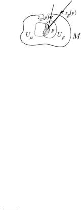
Fig. 2.15 The intersection of two local trivializations of a line bundle
ately construct a corresponding vector bundle. It suffices to use as transition functions the linear representation of the transition functions of the principal bundle:
ψαβ(V ) ≡ D ψαβ(G) Hom(V , V ) |
(2.4.20) |
For any vector bundle the dimension of the standard fibre is named the rank of the bundle.
Whenever the base-manifold of a fibre-bundle is complex and the transition functions are holomorphic maps, we say that the bundle is holomorphic.
A very important and simple class of holomorphic bundles are the line bundles. By definition these are principal bundles on a complex base manifold M with structural group C ≡ C\0, namely the multiplicative group of non-zero complex numbers.
Let zα (p) C be an element of the standard fibre above the point p Uα " Uβ M in the local trivialization α and let zβ (p) C be the corresponding fibre point in the local trivialization β. The transition function between the two trivialization is expressed by (see Fig. 2.15):
|
αβ (p) · zβ (p) |
zα (p) |
|
|||
zα (p) = f |
fαβ (p) = zβ (p) , = 0 |
(2.4.21) |
||||
|
|
|
|
|
C
2.5 Tangent and Cotangent Bundles
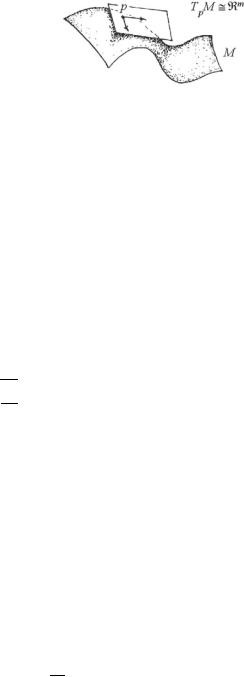
Let M be a differentiable manifold of dimension dim M = m: in Sect. 2.3 we have seen how to construct the tangent spaces TpM associated with each point p M of the manifold. We have also seen that each Tp M is a real vector space isomorphic to Rm. Considering the definition of fibre-bundles discussed in the previous section we now realize that what we actually did in Sect. 2.3 was to construct a vector-bundle, the tangent bundle T M (see Fig. 2.16).
In the tangent bundle T M the base manifold is the differentiable manifold M , the standard fibre is F = Rm and the structural group is GL(m, R) namely the group of real m × m matrices. The main point is that the transition functions are not newly introduced to construct the bundle rather they are completely determined from the transition functions relating open charts of the base manifold. In other words, whenever we define a manifold M , associated with it there is a unique vector bundle T M → M which encodes many intrinsic properties of M . Let us see how.
2.5 Tangent and Cotangent Bundles |
59 |
Fig. 2.16 The tangent bundle is obtained by gluing together all the tangent spaces
Consider two intersecting local charts (Uα , φα ) and (Uβ , φβ ) of our manifold. A tangent vector, in a point p M was written as:
|
|
|
∂ |
μ % |
|
|
tp |
= |
cμ(p) |
|
|
% |
(2.5.1) |
|
∂x |
|
%p |
|
||
|
|
|
|
% |
|
Now we can consider choosing smoothly a tangent vector for each point p M , namely introducing a map:
p M → tp Tp M |
(2.5.2) |
Mathematically what we have obtained is a section of the tangent bundle, namely a smooth choice of a point in the fibre for each point of the base. Explicitly this just means that the components cμ(p) of the tangent vector are smooth functions of the base point coordinates xμ. Since we use coordinates, we need an extra label denoting in which local patch the vector components are given:
t = c(α)μ (x) ∂x∂μ |p in chart α
(2.5.3)
t = c(β)ν (y) ∂y∂ν |p in chart β
having denoted xμ and yν the local coordinates in patches α and β, respectively. Since the tangent vector is the same, irrespectively of the coordinates used to describe it, we have:
c(β)ν (y) |
|
∂ |
= c(α)μ |
∂yν ∂ |
|||
|
(x) ∂xμ |
|
|||||
∂yν |
∂yν |
||||||
namely: |
|
|
|
|
|
|
|
cν |
(p) |
= |
cμ |
(p) ∂yν (p) |
|||
(β) |
|
|
(α) |
|
∂xμ |
(2.5.4)
(2.5.5)
In formula (2.5.5) we see the explicit form of the transition function between two local trivializations of the tangent bundle: it is simply the inverse Jacobian matrix associated with the transition functions between two local charts of the base mani-
"
fold M . On the intersection Uα Uβ we have:
|
|
|
# |
|
: |
|
→ |
|
= |
|
∂x |
(p) |
|
GL(m, R) |
(2.5.6) |
|
p |
|
Uα |
Uβ |
|
p |
|
ψβα (p) |
|
∂y |
|
as it is pictorially described in Fig. 2.17.