

174 |
4 Motion in the Schwarzschild Field |
shape of the orbit tends to restore part of the broken symmetry since the positions of the periastron and aphastron are symmetrically distributed on the unit circle.
4.4.1 Perturbative Treatment of the Periastron Advance
The orbits that we have obtained by numerical evaluation in the previous section are extremely far from the planetary orbits of the solar system. Indeed, in order to emphasize the phenomenon of the periastron advance we have chosen an orbit size of the order of tens of Schwarzschild emiradii while the actual order of magnitude of planetary orbits corresponds to hundred of millions of Schwarzschild emiradii. For Mercury, for instance, which is the innermost planet of the solar system, the Keplerian parameters have the following values:
aMercury = 55.46 × 10⁶ km
e = 0.2 |
(4.4.14) |
m6 = 1.4 km |
(Schwarzschild emiradius of the Sun) |
Large average radii means that u is small and the u2 term in (4.4.10) can be treated as a perturbation of the Newtonian differential (4.2.9). Let us therefore set:
u(φ) = u0(φ) + Δu(φ) |
(4.4.15) |
|||
where |
|
|
||
1 |
|
+ e cos φ) |
|
|
u0(φ) ≡ |
|
(1 |
(4.4.16) |
|
a(1 − e2) |
||||
is the unperturbed Newtonian solution of (4.2.9) and Δu(φ) u0(φ) is a small perturbation. Disregarding terms of order (Δu(φ))2, (4.4.7) becomes:
Δu + Δu = |
|
1 |
|
+ 3m(u0)2 |
a(1 |
− |
e2) |
||
|
|
|
|
2
= Hn cosn φ
n=0
where we have introduced the following constants:
3m
H0 = a2(1 − e2)2
6em H1 = a2(1 − e2)2
3e2m H2 = a2(1 − e2)2
(4.4.17)
(4.4.18)

4.4 The Periastron Advance |
175 |
Since (4.4.17) is linear in the unknown function Δu, its solution is the linear combination
2 |
|
Δu = Δun(φ) |
(4.4.19) |
n=0 |
|
where each term is the solution of an independent differential equation |
|
Δun + Δun = Hn cosn φ |
(4.4.20) |
Let us study the form of each Δun. The first contribution Δu0 is uninteresting and irrelevant since, for an arbitrary constant k, we have:
Δu0 = H0 + k cos φ |
(4.4.21) |
so that replacing u0 → u0 + Δu0 amounts to an unobservable renormalization of the Keplerian parameters a and e. Next we consider Δu2. Here a solution of the inhomogeneous equation is:
Δu2 = |
H2 |
− |
H2 |
cos 2φ |
(4.4.22) |
2 |
6 |
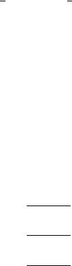
Also the perturbation u0 → u0 + Δu2 is essentially unobservable, since Δu2(φ) is periodic of period 2π . Indeed by replacing u0 → u0 + Δu2 we obtain a new orbit which is a slightly deformed ellipsis where the aphastro and periastro continue to occur at φ = 0 and φ = π as in the Keplerian case. This can be appreciated by looking at Figs. 4.13, 4.14, 4.15. In order to emphasize the extremely small effect of the perturbation we have chosen an ultra narrow and eccentric Keplerian orbit with parameters:
semilatus rectum = 8 Schwarzschild emiradii |
(4.4.23) |
eccentricity = 0.7 |
|
and in Fig. 4.13 we have compared the plot of the unperturbed function u0(φ) with the perturbed one u0(φ) + Δu2(φ). The resulting new orbit is plotted in Fig. 4.14 and compared with the unperturbed one. The periodic character of the perturbation implies that the new orbit looks like a deformed ellipsis of slightly changed shape and size. We can compare the actual shape of the perturbed orbit with a purely Keplerian ellipsis by defining a renormalized semilatus rectum and eccentricity via the formulae:
aR = r(π ) + r(0)
2
(4.4.24)
r(π ) − r(0) eR = +
r(π ) r(0)
where
1
r(φ) = (4.4.25) u0(φ) + Δu2(φ)
176 |
4 Motion in the Schwarzschild Field |
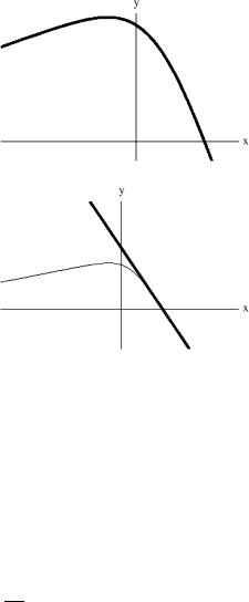
Fig. 4.13 Comparison of the unperturbed solution u0(φ) (thin line) and of the perturbed one
u0(φ) + Δu2(φ) (thick line) in the case of Keplerian parameters a = 8m, e = 0.7. As one sees, even in this extreme case of an ultra-narrow and ultra-relativistic orbit the perturbation modifies very slightly the shape of the function without changing its behavior and its periodicity
Fig. 4.14 Comparison of the Keplerian orbit of parameters a = 8m, e = 0.7 (thin line) with the perturbed orbit obtained by replacing
u0 → u0 + Δu2 (thick line)
Fig. 4.15 Comparison between a Keplerian orbit of parameters a = 8m, e = 0.7 perturbed by the periodic perturbation Δu2 (thick line) and a Keplerian orbit of parameters aR = 5.97683m, eR = 0.624945 (thin line) that, by definition, has the periastron and aphastron located at the same distances from the center of gravity as the perturbed orbit. This comparison shows the deviation from a purely elliptic shape
In Fig. 4.15 we have plotted the Keplerian orbit with parameters a = aR = 5.97683m, e = eR = 0.624945, together with the perturbed orbit of Keplerian parameters a = 8m, e = 0.7. By definition in these two orbits the aphastron and the
4.4 The Periastron Advance |
177 |
periastron are at the same distance, yet the first is a true ellipsis while the second, the perturbed orbit is not and it is slightly squashed. The change in shape is so small in actual astronomical situations where a 109m that the effect of the periodic perturbation Δu2 is absolutely unobservable.
We remain with the perturbation Δu1 that being non-periodic is the most interesting one. For n = 1 a solution of the inhomogeneous equation is:
|
|
|
|
Δu1 = |
H1 |
φ sin φ |
|
|
(4.4.26) |
|||
|
|
|
|
2 |
|
|
|
|||||
As long as: |
|
|
|
|
|
|
|
|
|
|
|
|
β |
≡ |
H1 |
|
|
a(1 − e2) |
|
|
3m |
|
1 |
(4.4.27) |
|
2 |
× |
|
= a(1 − e2) |
|
||||||||
|
|
e |
|
|
|
|
||||||
the interpretation of the perturbation u0 → Δu1 is simple. It suffices to note that under the condition (4.4.27) we can write:
|
cos (1 − β)φ cos φ + βφ sin φ + O β2 |
||||
in order to conclude that: |
|
|
|
||
u0 |
(φ) + Δu1(φ) |
1 |
|
1 + e cos (1 − β)φ |
|
a(1 |
e2) |
||||
|
|
− |
|
|
|
which is a periodic function of period |
|
|
|
||
|
|
T = |
2π |
> 2π |
|
|
|
1 β |
|||
|
|
|
− |
||
(4.4.28)
(4.4.29)
(4.4.30)
This means that at each revolution the periastron (and as a consequence the aphastron) occurs not at an angle 2π after the previous periastron rather after an angle T . For someone who looks at the sky this effect means that the angular position of the periastron advances of an angle:
Δφ = T − 2π = 2π |
1 |
− 1 |
2πβ = |
6π m |
(4.4.31) |
1 − β |
a(1 − e2) |
at each revolution.
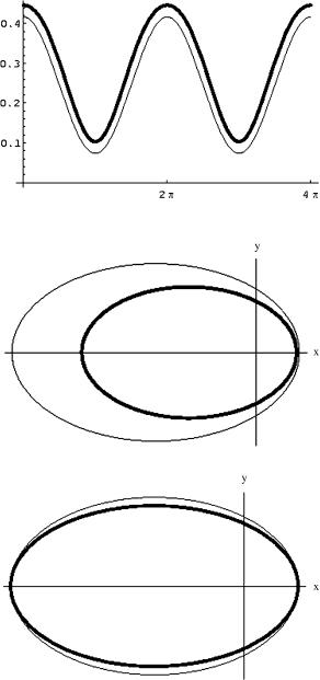
We can appreciate this phenomenon by means of numerical plots. As usual, in order to magnify the effect we choose a narrow relativistic orbit at a = 70m with eccentricity e = 0.6. In Fig. 4.16 we compare the plot of the unperturbed Keplerian solution u0(φ) with the perturbed solution u0(φ) + Δu1(φ) as interpreted in (4.4.29). The non-integer change in period is clearly seen in this plot. In Fig. 4.17 the classical Keplerian orbit u0(φ) and the perturbed one u0(φ) + Δu1(φ) are compared on several revolutions. Recalling Figs. 4.10, 4.11, 4.12 where we have plotted the numerical solution of the exact orbit differential equation at parameters a = 70m, e = 0.7 with Fig. 4.17 we see that the phenomenon of periastron advance featured
178 |
4 Motion in the Schwarzschild Field |
Fig. 4.16 Comparison of the unperturbed solution u0(φ) (thin line) and of the perturbed one
u0(φ) + Δu1(φ) (thick line) in the case of Keplerian parameters a = 70m, e = 0.6. The shift in period of the perturbed solution is evident from the plot
Fig. 4.17 Comparison of the unperturbed Keplerian orbit of parameters a = 70m,
e = 0.6 (thin line) with the orbit perturbed by
u0(φ) + Δu1(φ) (thick line). The phenomenon of the periastron advance is evident
by the exact solutions is essentially due to the non-periodic perturbation Δu1 of (4.4.26) as we have claimed.
Equation (4.4.31) is the final perturbative formula predicted by General Relativity for the periastron anomaly and constitutes one of the classical tests of the theory proposed by Einstein himself.
In the case of the solar system we have m = m6 = GM6/c2 where M6 is the solar mass. The same formula can also be applied to binary stellar systems. In this case we have:
G |
+ m2) |
|
mbinary c2 (m1 |
(4.4.32) |
where m1,2 denote the masses of the two companion stars.
It is interesting to insert the numerical values of the Keplerian parameters in the
case of the planet Mercury (see (4.4.14)). We obtain: |
|
|
|||||
ΔφMercury = 6π |
|
1.4 |
10−6 |
6π × 2.6 |
× 10−8 |
(4.4.33) |
|
|
|
|
|||||
0.96 |
× |
55.46 |
|||||
|
|
|
|
|
|
|
|
Since the period of Mercury is TMercury = 0.24 years it follows that in one terrestrial century we have 100/0.24 = 416.6 orbits of Mercury. On the other hand, if we

4.5 Light-Like Geodesics and the Deflection Light-Rays |
179 |
evaluate 6π in arc seconds we have:
6π = 3 × 60 × 60 × 360 arcs = 3, 888, 000 arcs |
(4.4.34) |
so that we can write:
ΔφMercury/century = 3, 888, 000 × 416.6 × 2.6 × 10−8 × arcs/century
42 /century |
(4.4.35) |
The value (4.4.35) is in perfect agreement with the historical records of astronomical observations after subtraction of all the Newtonian effects due to the perturbation on Mercury orbit by the motion of the other planets in the solar system.
4.5Light-Like Geodesics in the Schwarzschild Metric and the Deflection of Light Rays
Let us now go back to the Lagrangian (4.3.2) for time-like geodesics and replace it with its analogue for light-like geodesics. In this case we write:
|
L |
1 |
|
2 m dt 2 |
1 |
|
|
2 m −1 dr |
||||||||||||
− |
|
= − |
|
− |
|
|
r |
|
|
dλ |
|
+ |
|
− |
|
r |
|
dλ |
||
|
|
+ |
r2 |
|
dθ |
2 |
+ |
sin2 |
θ |
dφ |
2 |
|
|
|||||||
|
|
|
|
|
|
|||||||||||||||
|
|
|
|
dλ |
|
|
|
dλ |
|
|
|
|
||||||||
where λ is some affine parameter and we replace the constraint new one:
0 = dxμ dxν gμν (x) dλ dλ
2
(4.5.1)
2L = 1 with the
(4.5.2)
Just as in the case of time-like geodesics we can integrate the equation for the canonical variable θ by setting:
θ = |
π |
= const |
(4.5.3) |
2 |
In other words the trajectories of photons and massless particles are planar just as those of massive particles. Also in full analogy with the massive case we have that the canonical variables t and φ are cyclic and are respectively associated with two first integrals of the motion, the energy E and the angular momentum L. Explicitly we find:
dt |
1 − |
2m |
= E = const |
dλ |
r |
(4.5.4)
r2 dφ = L = const
dλ

180 |
4 Motion in the Schwarzschild Field |
Fig. 4.18 The effective radial potential for the motion of massless particles in Schwarzschild geometry. It displays a maximum at
r = 3m but no minima. In this
figure the plot is given for
L = 5
The difference with the massive case emerges when we enforce the new constraint (4.5.2) which yields the relation:
0 |
= |
|
|
E 2 |
|
|
|
|
|
|
|
|
r˙2 |
|
r2 |
L2 |
(4.5.5) |
|||||||
|
1 − |
2m |
− |
|
1 − |
2m |
− |
|
||||||||||||||||
|
|
|
|
|
r4 |
|
||||||||||||||||||
|
|
|
r |
r |
|
|
|
|||||||||||||||||
replacing (4.3.7). From (4.5.5) we obtain: |
|
|
|
|
|
|
|
|
|
|||||||||||||||
|
|
dr |
2 |
= |
E |
2 |
− |
V photon(r) |
|
|||||||||||||||
|
|
|
|
|
|
|
||||||||||||||||||
|
|
dλ |
|
|
|
|
|
|
eff |
|
|
|
|
(4.5.6) |
||||||||||
|
|
|
dφ |
|
|
|
|
L |
|
|
|
|
|
|
|
|
||||||||
|
|
|
= |
|
|
|
|
|
|
|
|
|
||||||||||||
|
|
|
|
|
|
|
|
|
|
|
|
|
|
|
|
|
||||||||
|
|
|
|
dλ |
r2 |
|
|
|
|
|
|
|
|
|
||||||||||
where the effective potential |
|
|
|
|
|
|
|
|
|
|
|
|
|
|
|
|
|
|
|
|
|
|
|
|
|
Veffphoton |
(r) = |
L2 |
|
− |
2mL2 |
|
(4.5.7) |
||||||||||||||||
|
r2 |
|
r3 |
|
||||||||||||||||||||
is the light-like counterpart of the massive effective potential (4.3.9). We can immediately note the differences. While the centrifugal barrier r12 is common to both
cases, the Newtonian attraction − 1r is absent in the light-like case. This corresponds to the obvious fact that in Newton’s theory photons do not feel gravity since they are massless. Yet the short range attractive correction due to General Relativity− r13 applies both to photons and massive particles. It is this correction which is responsible for the bending of light-rays in strong gravitational fields like that generated by the sun. This phenomenon is the light-like counterpart of the periastron
advance and constitutes another classical test of General Relativity. The plot of the potential Veffphoton(r) is displayed in Fig. 4.18. As it is evident from its shape there
is a maximum at r = 3m but no minima. Hence, in the case of photons there are no stable circular orbits: only open orbits are available that correspond to the aforementioned bending of light-rays. We study such a phenomenon by writing the exact differential equation of the orbit. Proceeding in full analogy with our previous treatment of the time-like geodesics we trade the derivatives with respect to the affine

4.5 Light-Like Geodesics and the Deflection Light-Rays |
181 |
parameter for the derivatives with respect to the azimuthal angle:
dr |
= |
dr dφ |
= |
dr L2 |
(4.5.8) |
||||
dλ |
dφ |
|
dλ |
dφ |
|
r2 |
|||
Inserting (4.5.8) into (4.5.6) and introducing the impact parameter:
|
|
|
|
|
|
|
L |
|
|
|
|
||
|
|
|
|
|
|
b ≡ E |
|
|
|
|
(4.5.9) |
||
we obtain: |
|
|
|
|
|
|
|
|
|
|
|
|
|
|
dr |
= ± |
r2 |
|
1 |
|
1 |
|
1 |
− |
2m |
1/2 |
(4.5.10) |
|
|
b2 |
− r2 |
|
|||||||||
dφ |
|
|
|
r |
|
||||||||
which can be further converted into the exact orbit equation:
du = ± |
|
b2 − |
|
+ |
|
−1/2 |
|
|
dφ |
|
1 |
|
u2 |
|
2mu3 |
(4.5.11) |
|
|
|
|
|
|||||
The name given to the impact parameter (4.5.9) is easily justified if we integrate (4.5.11) in the Newtonian approximation:
2mu3 u2
Indeed if we disregard the term 2mu3 we obtain:
|
dφ |
= ± |
|
|
|
du |
||
|
|
|
|
|||||
|
1 |
− u2 |
||||||
|
|
|
||||||
|
|
|
b2 |
|||||
which immediately yields:
φ + φ0 = arcsin[bu]
leading to the equation of the Newtonian orbit of a photon:
b
r =
sin[φ + φ0]
(4.5.12)
(4.5.13)
(4.5.14)
(4.5.15)
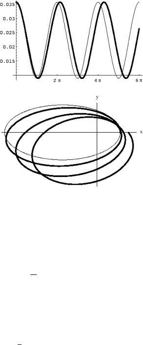
Equation (4.5.15) describes a straight line in the θ = π2 plane as it is shown in Fig. 4.19. The impact parameter b is geometrically interpreted as the minimal distance from the center of mass reached by the massless particle while traveling along its trajectory. Just as in the massive case, the relativistic perturbation 2mu3 changes this conclusion. Squaring both sides of (4.5.11) we obtain:
|
dφ |
2 |
− b2 − |
|
+ |
|
= |
|
|
|
|
du |
1 |
|
u2 |
|
2mu3 |
|
0 |
(4.5.16) |
|
|
|
|
|
|
||||||
182 |
4 Motion in the Schwarzschild Field |
Fig. 4.19 The Newtonian trajectory of a photon is a straight line and the impact parameter is the minimal distance from the center of mass reached along such a trajectory
and taking a further dφd derivative of (4.5.16) we find:
2u u + u − 3mu2 = 0 |
(4.5.17) |
which is solved either by u = 0 or by:
u + u = 3mu2 |
(4.5.18) |
The first possibility corresponding to circular orbits is excluded since, as we have already observed, the effective potential has no minima. Hence we are left with (4.5.18) which is the light-like counterpart of (4.4.10). Just as in the massive case the differential equation (4.5.18) can be either treated numerically or perturbatively, when the Newtonian approximation (4.5.12) applies. In order to emphasize the new relativistic phenomenon implied by Schwarzschild geometry, namely the gravitational bending of light rays, we have considered the extreme situation provided by a photon impinging on a center of mass with a tiny impact parameter, namely
b = 8.5 Schwarzschild emiradii |
(4.5.19) |
and choosing some non-vanishing incidence angle (φ0 = π/5 in our example) we have numerically solved (4.5.18) with initial conditions:
u (0) = |
sin φ0 |
; |
u(0) = |
cos φ0 |
(4.5.20) |
b |
b |
The resulting photon trajectory is displayed in Fig. 4.20. As one sees, rather than proceeding undisturbed on a straight line the photon makes a turn around the center of mass and emerges at an angle different from the one of incidence. The exact relativistic orbit is compared with the corresponding Newtonian one in Fig. 4.21.
4.5 Light-Like Geodesics and the Deflection Light-Rays |
183 |
Fig. 4.20 The trajectory of a photon in Schwarzschild geometry with impact parameter b = 8.5m and incidence angle φ0 = π5
Fig. 4.21 Comparison between the Newtonian trajectory (thick line) and the exact relativistic trajectory (thin line) of a photon that impinges a center of mass with impact parameter
b = 8.5m and incidence angle
φ0 = π5
The perturbative treatment of (4.5.18) follows the same lines as the perturbative treatment of orbit equation for the massive particle (4.4.10). We set
u(φ) = u0(φ) + Δu(φ) |
(4.5.21) |
||
where, according to (4.5.15), the unperturbed solution is: |
|
||
1 |
sin[φ + φ0] |
|
|
u0(φ) = |
|
(4.5.22) |
|
b |
|||
In the post-Newtonian approximation (4.5.12) we obtain the following differential equation for the perturbation:
Δu + Δu = 3mu02 = |
3m |
1 − cos2[φ + φ0] |
(4.5.23) |
b2 |
which admits the following particular solution:
|
= |
2b2 |
|
+ |
3 |
|
+ |
|
|
|
Δu(φ) |
|
3m |
1 |
|
1 |
cos 2(φ |
|
φ0) |
|
(4.5.24) |
|
|
|
|
|
Hence, choosing our reference frame orientation in such a way that φ0 = 0, we can write the perturbed solution:
|
= b |
[ |
|
] + |
b |
|
+ |
3 |
[ |
] |
|
upert(φ) |
1 |
sin |
φ |
|
3m |
1 |
|
1 |
cos 2φ |
|
(4.5.25) |
|
|
|
|
|

184 |
4 Motion in the Schwarzschild Field |
Fig. 4.22 Comparison between the Newtonian and post-Newtonian perturbed trajectory of a photon impinging on a center of mass with impact parameter
b = 30m and incidence angle
φ0 = 0
The corresponding trajectory is plotted in Fig. 4.22 for an impact parameter b = 30m. In the same figure we have also plotted the corresponding Newtonian trajectory, namely a straight-line with the same minimal distance from the center of mass. The angle δ shown in Fig. 4.22 is one half of the total deflection angle of light rays predicted by General Relativity:
Δφlight = 2|δ| |
(4.5.26) |
The angle δ can be evaluated from the post-Newtonian perturbed solution (4.5.25) with the following reasoning. The incoming and outgoing photons are at infinite distance from the center of mass, namely at r = ∞ u = 0. If we fix φ0 = 0, the zeros of the unperturbed function u0(φ) (see (4.5.22)), are at:
r |
= ∞ |
u0 |
= |
0 |
|
φ(0) |
= |
|
0 |
incoming photon |
(4.5.27) |
|
|
|
∞ |
|
π |
outgoing photon |
|
The zeros of the perturbed function will instead occur at:
r |
|
upert 0 |
φ(pert) |
|
0 |
− δ |
incoming photon (4.5.28) |
|
|
= ∞ |
= |
∞ |
= |
π |
+ |
δ |
outgoing photon |
|
|
|||||||
where δ 1 is small. Hence we can use the power series expansion of trigonometric functions and write:
|
sin φ∞ φ∞ = δ; |
|
|
cos 2φ∞ 1 |
(4.5.29) |
|||||||||||
and write |
|
|
|
|
|
|
|
|
|
|
|
|
|
|
|
|
0 |
|
δ |
+ |
|
3m |
1 |
+ |
1 |
|
|
δ |
= |
2 |
m |
(4.5.30) |
|
= − b |
2b2 |
3 |
b |
|||||||||||||
|
|
|
|
|
|
|||||||||||
Inserting (4.5.30) into (4.5.26) we conclude that General Relativity predicts the following total deflection angle