

44 |
2 Manifolds and Fibre Bundles |
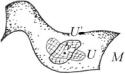
Fig. 2.6 A germ of a smooth |
|
function is the equivalence |
|
class of all locally defined |
|
function that coincide in some |
|
neighborhood of a point p |
|
Definition 2.2.8 Given a point p M , the space of germs of smooth functions at p, denoted C∞p is defined as follows. Consider all the open neighborhoods of p, namely all the open subsets Up M such that p Up . Consider the space of smooth functions C∞(Up ) on each Up . Two functions f C∞(Up ) and g C∞(Up ) are said to be equivalent if they coincide on the intersection Up
(see Fig. 2.6):
f |
|
g |
|
| |
|
" |
= |
| |
|
" |
|
(2.2.26) |
|
|
f U |
p |
U |
p |
g U |
p |
U |
p |
|||
|
|
|
|
|
|
|
|
|
The union of all the spaces C∞(Up ) modded by the equivalence relation (2.2.26) is the space of germs of smooth functions at p:
Cp∞ ≡ |
Up |
C∞(Up) |
(2.2.27) |
|
|
||
|
|
|
What underlies the above definition of germs is the familiar principle of analytic continuation. Of the same function we can have different definitions that have different domains of validity: apparently we have different functions but if they coincide on some open region than we consider them just as different representations of a single function. Given any germ in some open neighborhood Up we try to extend it to a larger domain by suitably changing its representation. In general there is a limit to such extension and only very special germs extend to globally defined functions on the whole manifold M . For instance the power series k N zk defines a holomorphic function within its radius of convergence |z| < 1. As everybody knows, within the convergence radius the sum of this series coincides with 1/(1 − z) which is a holomorphic function defined on a much larger neighborhood of z = 0. According to our definition the two functions are equivalent and correspond to two different representatives of the same germ. The germ, however, does not extend to a holomorphic function on the whole Riemann sphere C ∞ since it has a singularity in z = 1. Indeed, as stated by Liouville theorem, the space of global holomorphic functions on the Riemann sphere contains only the constant function.
2.3 Tangent and Cotangent Spaces
In elementary geometry the notion of a tangent line is associated with the notion of a curve. Hence to introduce tangent vectors we have to begin with the notion of curves in a manifold.
2.3 Tangent and Cotangent Spaces |
45 |
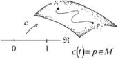
Fig. 2.7 A curve in a manifold is a continuous map of an interval of the real line into the manifold itself
Definition 2.3.1 A curve C in a manifold M is a continuous and differentiable map of an interval of the real line (say [0, 1] R) into M :
C : [0, 1] → M |
(2.3.1) |
In other words a curve is one-dimensional submanifold C M (see Fig. 2.7). |
|
There are curves with a boundary, namely C (0) |
C (1) and open curves that do |
not contain their boundary. This happens if in (2.3.1) we replace the closed interval [0, 1] with the open interval ]0, 1[. Closed curves or loops correspond to the case where the initial and final point coincide, that is when pi ≡ C (0) = C (1) ≡ pf . Differently said
Definition 2.3.2 A closed curved is a continuous differentiable map of a circle into the manifold:
C : S1 → M |
(2.3.2) |
Indeed, identifying the initial and final point means to consider the points of the curve as being in one-to-one correspondence with the equivalence classes
R/Z ≡ S1 |
(2.3.3) |
which constitute the mathematical definition of the circle. Explicitly (2.3.3) means that two real numbers r and r are declared to be equivalent if their difference r − r = n is an integer number n Z. As representatives of these equivalence classes we have the real numbers contained in the interval [0, 1] with the proviso that 0 1.
We can also consider semiopen curves corresponding to maps of the semiopen interval [0, 1[ into M . In particular, in order to define tangent vectors we are interested in open branches of curves defined in the neighborhood of a point.
2.3.1 Tangent Vectors in a Point p M
For each point p M let us fix an open neighborhood Up M and let us consider the semiopen curves of the following type:
$
Cp : [0, 1[→ Up
(2.3.4)
Cp (0) = p
46 |
2 Manifolds and Fibre Bundles |
Fig. 2.8 In a neighborhood Up of each point p M we consider the curves that go through p
Fig. 2.9 The tangent space in a generic point of an S2 sphere
In other words for each point p let us consider all possible curves Cp (t) that go trough p (see Fig. 2.8).
Intuitively the tangent in p to a curve that starts from p is the vector that specifies the curve’s initial direction. The basic idea is that in an m-dimensional manifold there are as many directions in which the curve can depart as there are vectors in Rm: furthermore for sufficiently small neighborhoods of p we cannot tell the difference between the manifold M and the flat vector space Rm. Hence to each point p M of a manifold we can attach an m-dimensional real vector space
p M : p → Tp M dim TpM = m |
(2.3.5) |
which parameterizes the possible directions in which a curve starting at p can depart. This vector space is named the tangent space to M at the point p and is, by definition, isomorphic to Rm, namely Tp M Rm. For instance to each point of an S2 sphere we attach a tangent plane R2 (see Fig. 2.9).
Let us now make this intuitive notion mathematically precise. Consider a point p M and a germ of smooth function fp Cp∞(M ). In any open chart (Uα , ϕα ) that contains the point p, the germ fp is represented by an infinitely differentiable function of m-variables:
fp x(α)1 , . . . , x(α)m |
(2.3.6) |
|||
Let us now choose an open curve Cp (t) that lies in Uα and starts at p: |
|
|||
$Cp |
0, 1 |
[→ |
Uα |
(2.3.7) |
Cp(t) : |
: [ |
|
||
Cp (0) = p |
|
|
||
and consider the composite map: |
|
|
|
|
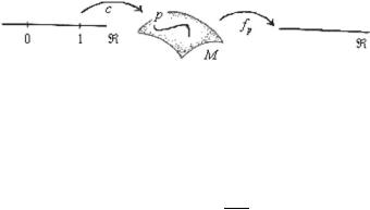
fp ◦ Cp : |
[0, 1[ R → R |
(2.3.8) |
||
which is a real function |
|
|
|
|
fp Cp (t) ≡ gp (t) |
(2.3.9) |
|||
of one real variable (see Fig. 2.10). |
|
|
|
|
2.3 Tangent and Cotangent Spaces |
47 |
Fig. 2.10 The composite map fp ◦ Cp where fp is a germ of smooth function in p and Cp is a curve departing from p M
We can calculate its derivative with respect to t in (Uα , ϕα ), reads as follows:
d |
gp (t)% |
|
0 = |
∂fp |
· |
dxμ |
|
|
|
|
μ |
|
|||
dt |
% |
|
∂x |
dt |
|||
%t |
= |
|
|||||
|
% |
|
|
|
|
|
|
t = 0 which, in the open chart
%
%
% (2.3.10)
%t=0
We see from the above formula that the increment of any germ fp C∞p (M ) along a curve Cp (t) is defined by means of the following m real coefficients:
cμ |
≡ |
dxμ % |
|
|
|
|
R |
(2.3.11) |
|||||
|
|
|
% |
|
|
|
|
|
|
||||
|
|
|
dt |
%t |
= |
0 |
|
|
|
||||
|
|
|
|
% |
|
|
|
|
|
= |
|||
which can be calculated whenever the parametric form of the curve is given: xμ |
|||||||||||||
xμ(t). Explicitly we have: |
|
|
|
|
|
|
|
|
|
|
|
||
|
dfp |
= cμ |
|
∂fp |
|
(2.3.12) |
|||||||
|
|
|
|
|
|
|
|
||||||
|
|
dt |
|
|
∂xμ |
|
|||||||
Equation (2.3.12) can be interpreted as the action of a differential operator on the space of germs of smooth functions, namely:
|
≡ |
∂xμ |
|
|
|
|
: |
|
p |
|
|
→ |
p |
|
||||
tp |
|
cμ |
∂ |
|
|
|
|
tp |
|
C∞(M ) |
|
C∞(M ) |
(2.3.13) |
|||||
|
|
|
|
|
|
|
|
|||||||||||
Indeed for any germ f and for any curve |
|
|
|
|
|
|
|
|
|
|||||||||
|
|
tp f |
= |
dxμ |
% |
|
|
∂f |
|
|
C∞(M ) |
(2.3.14) |
||||||
|
|
|
|
|
|
|
μ |
|||||||||||
|
|
|
|
dt |
% |
|
0 ∂x |
p |
|
|
|
|||||||
|
|
|
|
%t |
= |
|
|
|
|
|
|
|||||||
|
|
|
|
|
|
|
% |
|
|
|
|
|
|
|
|
|
|
|
is a new germ of a smooth function in the point p. This discussion justifies the mathematical definition of the tangent space:
Definition 2.3.3 The tangent space Tp M to the manifold M in the point p is the
vector space of first order differential operators on the germs of smooth functions
C∞p (M ).
Next let us observe that the space of germs C∞p (M ) is an algebra with respect to linear combinations with real coefficients (αf + βg)(p) = αf (p) + βg(p) and pointwise multiplication f · g(p) ≡ f (p)g(p):
48 |
|
|
|
|
|
|
|
|
|
|
|
|
2 Manifolds and Fibre Bundles |
|
|
α, β |
|
|
|
f, g |
|
p |
αf |
+ |
βg |
|
p |
|
|
|
|
R |
|
|
C∞(M ) |
|
|
C∞(M ) |
|
|||||
|
|
|
|
f, g |
p |
|
f |
· |
g |
p |
(2.3.15) |
|||
|
|
|
|
|
|
C∞(M ) |
|
|
|
C∞(M ) |
||||
(αf + βg) · h = αf · h + βg · h
and a tangent vector tp is a derivation of this algebra.
Definition 2.3.4 A derivation D of an algebra A is a map: |
|
||
|
|
D : A → A |
(2.3.16) |
that |
|
|
|
1. |
is linear |
|
|
|
α, β R f, g A : |
D (αf + βg) = αD f + βD g |
(2.3.17) |
2. |
obeys Leibnitz rule |
|
|
|
f, g A : |
D (f · g) = D f · g + f · D g |
(2.3.18) |
That tangent vectors fit into Definition 2.3.4 is clear from their explicit realization as differential operators (2.3.13), (2.3.14). It is also clear that the set of derivations D[A ] of an algebra constitutes a real vector space. Indeed a linear combination of derivations is still a derivation, having set:
α, β R, D1, D2 D[A ], f A : (αD1 + βD2)f = αD1f + βD2f
(2.3.19)
Hence an equivalent and more abstract definition of the tangent space is the following:
Definition 2.3.5 The tangent space to a manifold M at the point p is the vector space of derivations of the algebra of germs of smooth functions in p:
Tp M ≡ D Cp∞(M ) |
(2.3.20) |
Indeed for any tangent vector (2.3.13) and for any pair of germs f, g C∞p (M ) we have:
tp (αf + βg) = αtp (f ) + βtp (g)
(2.3.21)
tp (f · g) = tp (f ) · g + f · tp (g)
In each coordinate patch a tangent vector is, as we have seen, a first order differential operator singled out by its components, namely by the coefficients cμ. In the language of tensor calculus the tangent vector is identified with the m-tuplet of real numbers cμ. The relevant point, however, is that such m-tuplet representing the
2.3 Tangent and Cotangent Spaces |
49 |
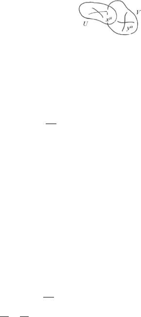
Fig. 2.11 Two coordinate patches
same tangent vector is different in different coordinate patches. Consider two coordinate patches (U, ϕ) and (V , ψ) with non-vanishing intersection. Name xμ the coordinate of a point p U " V in the patch (U, ϕ) and yα the coordinate of the same point in the patch (V , ψ). The transition function and its inverse are expressed by setting:
xμ = xμ(y); |
yν = yν (x) |
(2.3.22) |
Then the same first order differential operator can be alternatively written as:
tp |
= |
cμ |
∂ |
or tp |
= |
cμ |
∂yν |
∂ |
= |
cν |
∂ |
(2.3.23) |
|||
|
∂yν |
∂yν |
|||||||||||||
|
∂xμ |
|
|
|
|
∂xμ |
|
|
|||||||
having defined: |
|
|
|
|
|
|
|
|
|
|
|
|
|
|
|
|
|
|
|
cν |
≡ |
cμ |
∂yν |
|
|
|
|
|
(2.3.24) |
||
|
|
|
|
|
|
|
|
|
|||||||
|
|
|
|
|
|
|
∂xμ |
|
|
|
|
|
|||
Equation (2.3.24) expresses the transformation rule for the components of a tangent vector from one coordinate patch to another one (see Fig. 2.11).
Such a transformation is linear and the matrix that realizes it is the inverse of the Jacobian matrix (∂y/∂x) = (∂x/∂y)−1. For this reason we say that the components of a tangent vector constitute a controvariant world vector. By definition a covariant world vector transforms instead with the Jacobian matrix. We will see that covariant world vectors are the components of a differential form.
2.3.2 Differential Forms in a Point p M
Let us now consider the total differential of a function (better of a germ of a smooth
function) when we evaluate it along a curve. |
|
f |
|
|
p |
|
|
||||||||
|
|
|
C∞(M ) and for each curve c(t) |
||||||||||||
starting at p we have: |
|
|
|
|
|
|
|
|
|
|
|
|
|
|
|
|
dt |
|
|
% |
|
= |
|
∂xμ |
|
|
≡ |
|
|
||
|
d |
f |
c(t) |
% |
|
|
cμ |
|
∂ |
|
f |
|
tpf |
(2.3.25) |
|
|
|
|
|
%t |
= |
0 |
|
|
|
|
|
|
|
|
|
|
|
|
|
% |
|
|
|
|
|
|
|
|
|
|
|
where we have named tp = dcdtμ |t=0 ∂x∂μ the tangent vector to the curve in its initial point p. So, fixing a tangent vector means that for any germ f we know its total differential along the curve that admits such a vector as tangent in p. Let us now reverse our viewpoint. Rather than keeping the tangent vector fixed and letting the germ f vary let us keep the germ f fixed and let us consider all possible curves that
50 |
2 Manifolds and Fibre Bundles |
depart from the point p. We would like to evaluate the total derivative of the germ dfdt along each curve. The solution of such a problem is easily obtained: given the tangent vector tp to the curve in p we have df/dt = tp f . The moral of this tale is the following: the concept of total differential of a germ is the dual of the concept of tangent vector. Indeed we recall from linear algebra that the dual of a vector space is the space of linear functionals on that vector space and our discussion shows that the total differential of a germ is precisely a linear functional on the tangent space Tp M .
Definition 2.3.6 The total differential dfp of a smooth germ f |
|
p |
|
|
C∞(M ) is a |
||
linear functional on Tp M such that |
|
|
|
tp Tp M |
dfp (tp ) = tp f |
|
(2.3.26) |
tp , kp Tp M , α, β R |
dfp (αtp + βkp ) = αdfp (tp ) + βdfp (kp) |
||
The linear functionals on a finite dimensional vector space V constitute a vector space V (the dual) with the same dimension. This justifies the following
Definition 2.3.7 We name cotangent space to the manifold M in the point p the vector space Tp M of linear functionals (or 1-forms in p) on the tangent space
Tp M :
|
|
|
|
p |
≡ |
Hom(T |
p |
M , R) |
= |
(T |
p |
M ) |
(2.3.27) |
|
|
|
|
T M |
|
|
|
|
|||||
|
So we name differential 1-forms in p the elements of the cotangent space and |
||||||||||||
|
|
|
p |
|
|
|
|
|
|
|
|
|
|
|
ωp |
|
T |
M we have: |
|
|
|
|
|
|
|
|
|
1) tp Tp M : |
|
ωp (tp ) R |
|
|
|
|
(2.3.28) |
||||||
2) α, β R, tp , kp Tp M : ωp (αtp + βkp ) = αωp(tp ) + βωp (kp) |
|
||||||||||||
The reason why the above linear functionals are named differential 1-forms is that in every coordinate patch {xμ} they can be expressed as linear combinations of the coordinate differentials:
|
|
ωp = ωμ dxμ |
(2.3.29) |
and their action on the tangent vectors is expressed as follows: |
|
||
tp = cμ |
∂ |
ωp(tp ) = ωμcμ R |
(2.3.30) |
|
|||
∂xμ |
|||
Indeed in the particular case where the 1-form is exact (namely it is the differential of a germ) ωp = dfp we can write ωp = ∂f/∂xμ dxμ and we have dfp (tp ) ≡ tp f = cμ∂f/∂xμ. Hence when we extend our definition to differential forms that are not exact we continue to state the same statement, namely that the value of the 1-form on a tangent vector is given by (2.3.30).