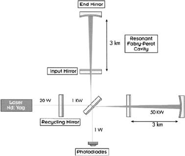
Fig. 7.5 The schema of a gravitational interferometer

disturbance should deform the lengths and should be revealed by the sudden appearance of an interference.

At the present time two gravitational interferometers are in operation and a third is under construction. The existing machines are Virgo, located near Pisa, and Ligo I, located in Louisiana, US. The third machine Ligo II is being built in the Washington State, US.

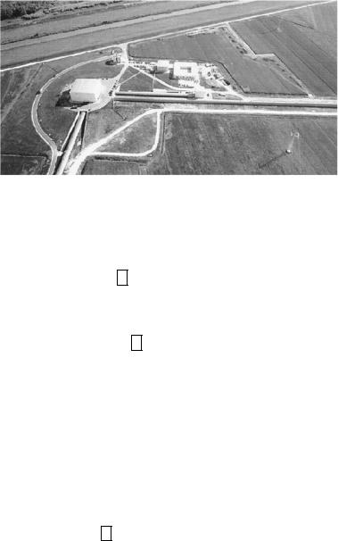
The first six months of joint observations by Virgo (see Fig. 7.6) and Ligo I took place about two years ago and so far no event of gravitational wave transit was detected. The direct detection of the elusive waves is just postponed. All experimentalists in this field share the view that a further effort to increase the already fantastic sensitivity of their instrument is necessary, unless we are specially lucky and a binary coalescence suddenly takes place rather closely to us.

This being the status of observations let us now carefully consider the mathematical derivation of gravitational wave emission in the weak field approximation of Einstein theory. A systematic treatment of this problem necessarily begins with a discussion of Green functions, namely the inverse of the d’Alembertian wave operator.

7.2 Green Functions

The mathematical problem associated with all cases of relativistic wave propagation is that of inverting the d’Alembertian operator:

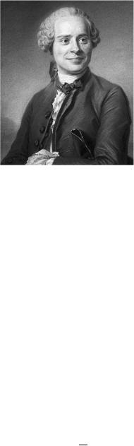
Fig. 7.7 Jean Baptiste Le Rond D’Alembert (1717–1783). D’Alembert was born and died in Paris. Illegitimate child of a writer noble-woman and of an officer, he was abandoned by his mother on the steps of the church of St.Jean Le Rond. Raised in an adoptive humble family he was educated by Jansenists in the Collège des Quatre-Nations at the expenses of his natural father who secretly left him an annuity. One among the top figures of the XVII century enlightenment, d’Alembert who invented such a name for himself was a mathematician, a physicist, a philosopher and a man of letters. Member of the French Academy of Sciences, friend and collaborator of Denis Diderot and of many other philosophers of that age he gave outstanding contributions in mathematics, mechanics and optics. He was member of the team preparing the Encyclopedie of which he wrote more than a thousand articles. The differential equation of wave propagation: ∂2f/∂t2 − ∂2f/∂x2 = 0 is one among his many fundamental contributions

where k2 ≡ kμkμ is the Lorentzian norm of the momentum vector kμ. This leads to the following solution for the Green function:

The problem with (7.2.4) is that it is singular since there is a pole along the integration path. The recipe to avoid such a singularity can be provided in three different ways and this leads to three different solutions for the Green function, having distinct physical properties and distinct uses: the advanced, retarded and Feynman

propagators. In order to appreciate the bearing of Lorentz signature we compare with the solution of the analogue problem in Euclidian signature, namely with the construction of the Green function for the Laplace operator.

7.2.1 The Laplace Operator and Potential Theory

In potential theory for the case of Newtonian or Coulomb forces, one is confronted with a similar problem, the inversion of the Laplace operator:

we can calculate the potential V (x) generated by an arbitrary distribution of masses or charges ρ(x):

In a completely analogous way to the relativistic case we obtain the integral representation of the Laplace Green function that follows: