70 2 Manifolds and Fibre Bundles

Z(f ). This differential form is named the total differential of the function f . In a local chart U with local coordinates x1, . . . , xm we have:

More generally we can see that there exists an endomorphism d, (ω → dω) of A (M ) onto itself with the following properties:

In each local coordinate patch the above intrinsic definition of the exterior differential leads to the following explicit representation:

As already stressed the exterior differential is the generalization of the concept of curl, well known in elementary vector calculus.

In the next section we introduce the notions of homotopy, homology and cohomology that are crucial to understand the global properties of manifolds and Lie groups and will also play an important role in formulating supergravity.

2.6 Homotopy, Homology and Cohomology

Differential 1-forms can be integrated along differentiable paths on manifolds. The higher differential p-forms, to be introduced shortly from now, can be integrated on p-dimensional submanifolds. An appropriate discussion of such integrals and of their properties requires the fundamental concepts of algebraic topology, namely homotopy and homology. Also the global properties of Lie groups and their many- to-one relation with Lie algebras can be understood only in terms of homotopy. For this reason we devote the present section to an introductory discussion of homotopy, homology and of its dual, cohomology.

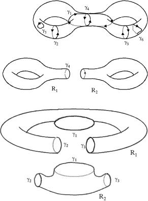
The kind of problems we are going to consider can be intuitively grasped if we consider Fig. 2.20, displaying a closed two-dimensional surface with two handles (actually an oriented, closed Riemann surface of genus g = 2) on which we have drawn several different closed 1-dimensional paths γ1, . . . , γ6.

Consider first the path γ5. It is an intuitive fact that γ5 can be continuously deformed to just a point on the surface. Paths with such a property are named homotopically trivial or homotopic to zero. It is also an intuitive fact that neither γ2, nor γ3, nor γ1, nor γ4 are homotopically trivial. Paths of such a type are homotopically

Fig. 2.20 A closed surface with two handles marked by several different closed 1-dimensional paths

Fig. 2.21 When we cut a surface along a path that is a boundary, namely it is homologically trivial, the surface splits into two separate parts

Fig. 2.22 The sum of the three paths γ1, γ2, γ3 is homologically trivial, namely γ2 + γ3 is homologous to −γ1

non-trivial. Furthermore we say that two paths are homotopic if one can be continuously deformed into the other. This is for instance the case of γ6 which is clearly homotopic to γ3.

Let us now consider the difference between path γ4 and path γ1 from another viewpoint. Imagine the result of cutting the surface along the path γ4. After the cut the surface splits into two separate parts, R1 and R2 as shown in Fig. 2.21. Such a splitting does not occur if we cut the original surface along the path γ1. The reason for this different behavior resides in this. The path γ4 is the boundary of a region on the surface (the region R1 or, equivalently its complement R2) while γ1 is not the boundary of any region. A similar statement is true for the paths γ2 or γ3. We say that γ4 is homologically trivial while γ1, γ2, γ3 are homologically non-trivial.

Next let us observe that if we simultaneously cut the original surface along γ1, γ2, γ3 the surface splits once again into two separate parts as shown in Fig. 2.22.

This is due to the fact that the sum of the three paths is the boundary of a region: either R1 or R2 of Fig. 2.22. In this case we say that γ2 + γ3 is homologous to −γ1, since the difference γ2 + γ3 − (−γ3) is a boundary.

In order to give a rigorous formulation to these intuitive concepts,which can be extended also to higher dimensional submanifolds of any manifold we proceed as follows.

Fig. 2.23 Two paths with coinciding extrema

In particular if σ is a closed path, namely a loop at x0, i.e. if x0 = x1 and if τ

then we say that σ is homotopically trivial and that it can be contracted to a point. It is quite obvious that the homotopy relation σ τ is an equivalence relation.

Hence we shall consider the homotopy classes [σ ] of paths from x0 to x1.

Next we can define a binary product operation on the space of paths in the following way. If σ is a path from x0 to x1 and τ is a path from x1 to x2 we can define a path from x0 to x2 traveling first along σ and then along τ . More precisely we set:

then σ τ σ τ . The proof is immediate and it is left to the reader. Hence without any ambiguity we can multiply the equivalence class of σ with the equivalence class of τ always assuming that the final point of σ coincides with the initial point of τ . Relying on these definitions we have a theorem which is very easy to prove but has an outstanding relevance:

Theorem 2.6.1 Let π1(M , x0) be the set of homotopy classes of loops in the manifold M with base in the point x0 M . If the product law of paths is defined as we just explained above, then with respect to this operation π1(M , x0) is a group whose identity element is provided by the homotopy class of the constant loop at x0 and the inverse of the homotopy class [σ ] is the homotopy class of the loop σ −1 defined by:

(In other words σ −1 is the same path followed backward.)

Proof Clearly the composition of a loop σ with the constant loop (from now on denoted as x0) yields σ . Hence x0 is effectively the identity element of the group. We still have to show that σ σ −1 x0. The explicit realization of the required homotopy is provided by the following function:

Therefore it is sufficient to check that F (s, t) is continuous. Dividing the square [0, 1] × [0, 1] into three triangles as in Fig. 2.24 we see that F (s, t) is continuous in each of the triangles and that is consistently glued on the sides of the triangles. Hence F as defined in (2.6.11) is continuous. This concludes the proof of the theo-

From this theorem it follows that in a arc-wise connected manifold, namely in a manifold where every point is connected to any other by at least one piece-wise differentiable path, the group π1(M , x0) is independent from the choice of the base point x0 and we can call it simply π1(M ). The group π1(M ) is named the first homotopy group of the manifold or simply the fundamental group of M .