4.3.1 Extrema of the Effective Potential and Circular Orbits

potential. Hence, just as in classical Newtonian mechanics we have to study the extrema of the effective potential (4.3.9) in order to establish the conditions for stable and unstable circular orbits. Indeed if an orbit is circular we have dτdr = 0 and the radius r = r0 must be a root of the equation Veff (r) = E . The orbit will be stable if r0 is a minimum of the effective potential Veff , while it will be unstable if it is a maximum. Equating to zero the first derivative of Veff we obtain:

there are no extrema and consequently no stable orbits. Reinstalling physical units the stability bound (4.3.19) translates into:

where T and R are the period and radius of the orbit, respectively, and M6 denotes the mass of the sun. Inserting the numerical values of these physical constants we find:

Therefore the critical limit in the solar system is given by:

It is instructive to compare condition (4.3.23) with the actual values of planetary radii or periods. The period of a planet is of the order of the year. Hence to be critical the radius of the orbit should be of the order of 10−2 km while, as we know, the typical distance of a planet from the sun is of the order of 108 km. Alternatively keeping the distance fixed, for instance inserting the average radius of the Earth orbit around the Sun:

we obtain that a critical period for such a orbit would be Tcrit = 1020 years. In other words, in order to be critical, the Earth should be so slow as to make a full revolution in a time ten orders of magnitude longer than the age of the Universe

TUniverse ≈ 1010 years.

These numerical considerations give some appreciation of how far the solar system is from the critical phenomena implied by general relativity and explain why Newtonian mechanics works so well for the physical system it was invented to explain. Notwithstanding this smallness, the critical region is by no means irrelevant in astrophysical systems. Indeed, as we are going to see, it becomes quite important near compact stars whose mass is of the order of a stellar mass M6 but whose radius is of the order of the kilometer.

Minimum and Maximum The second derivative of the potential yields:

The important conclusion that we reach from (4.3.27) is that stable orbits exist only for radii r > 6m. In the case of the Sun the numerical value of the Schwarzschild emiradius reads:

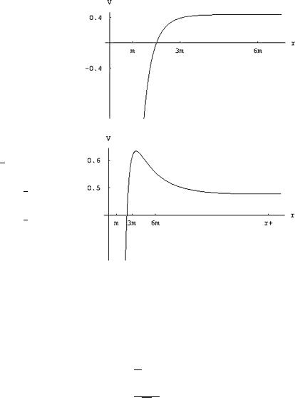
Fig. 4.6 Schwarzschild geometry: Plot of the

effective radial potential for= 1 L2 = 12m2. This is

the limiting case where no circular orbits are available. Indeed the potential has no extrema

Fig. 4.7 Schwarzschild geometry: Plot of the

effective√ potential for= 2 L2 = 24m2.

In this case the stable minimum of√the potential is at r+ = 6(2+ 2)m = 20.4853m, while the unstable

maximum is√at

r− = 6(2− 2)m = 3.51472m

It follows that the range of the root r− is:

and that is the range where unstable circular orbits are present.

In view of this analysis it is convenient to define the following dimensionless variables:

ρ = r m

(4.3.31)

= √ L

12m

and rewrite the effective potential (4.3.9) in terms of these:

The structure of the effective potential can be visualized by means of some plots. In Fig. 4.6 we display the limiting case L2 = 12m2 which admits no circular orbits. The reason is evident from the shape. In this case the potential has neither minima nor maxima. It just decreases from infinity towards infinitely large negative values