Fig. 3.1 A symbolic assessment by C.N. Yang that Mathematics and Physics have a common root

3.2 A Historical Outline

One spring in the late seventies, C.N. Yang, the father of gauge-theories and one among the most extraordinary scientific minds of the XXth century, was invited by Scuola Normale di Pisa to give the traditional yearly series of Fermian Lectures. It was just the eve of the 1983 experimental discovery of the W and Z bosons, which finally confirmed that gauge theories are indeed the language adopted by Nature to express the fundamental forces binding matter together and driving the evolution of the physical world. Yang chose to start his recollection of gauge-theories and his personal assessment of the entire subject from a symbolic picture of the kind shown in Fig. 3.1.

Two leaves depart from the same stem: one is Mathematics, the other is Physics. The two leaves live parallel lives but have a common root and, as it happens in non-Euclidian geometry, parallels can and indeed do intersect. They frequently intersect and, equally frequently, interchange the role of guiding pivot. Examples are numberless both in recent and less recent history of science. This is a relevant but somehow trivial observation.

The most profound allusion in the typical Chinese symbolism of Yang’s picture is the common stem of the two leaves. Mathematics and Physics were not that much socially and academically separated in the XIXth as they became in the XXth century and were further unified by a common denominator: the shared philosophical attitude of both the mathematician and the physicist, the latter assessing himself a natural philosopher.

The common root of Modern Mathematics and Modern Theoretical Physics is most prominently evident in the case of the concepts of connections and metrics which constitute the main topics of the present chapter. From the physical side these mathematical notions encode all the fundamental interactions among elementary matter constituents. From the mathematical side they are the corner stones of Differential Geometry, Algebraic Topology and allied subjects.

The historical developments of both the notion of a connection and the notion of a metric are quite long, spreading over more than a century. They are strongly intertwined and involve both Physics and Mathematics in an alternate and entangled fashion.

Two fundamental geometrical problems are at the basis of both notions: the problem of length and the problem of parallel transport, namely how can we measure

distances in a general continuous space and how do we assess the parallelism of two lines going through different points of that space. It turns out that these two apparently different problems are intimately related. Such a relation is the reason why connections and metrics, although genuinely different and independent mathematical notions can be, under certain conditions, related in a one-to-one fashion. The case where connection and metric are one-to-one related corresponds to Gravity and is the play-ground of General Relativity, while the case where the connection stands on his own feet is the case of non-gravitational interactions and encodes all the rest of Physics.

Historically the first notion of connection that was discovered is that of the metric connection named after its systematizer, the Italian mathematician Levi Civita. The Levi Civita connection is that appropriate to a Riemannian manifold, namely to a manifold equipped with a metric and it is analytically described by the 3-index symbols { νρμ }, introduced in the XIXth century by their German inventor, Elwin Bruno Christoffel. The development of such a notion is embedded in the development of Riemannian geometry, embracing the fall of the XIXth century and the dawn of the XXth, which is a mathematical tale strongly intertwined with the physical tale of Einstein’s quest for General Covariance and the Theory of Gravity.

It took several decades in the first half of the XXth century and the work of several mathematicians to single out the notion of a connection on a principal fibre bundle, purified from association with a metric. In a completely independent way in 1954 Yang and Mills introduced the physical notion of non-Abelian gauge fields which extends to all Lie groups G the structure of the electromagnetic theory based on the simplest of all such groups, namely U(1). In the course of due time the mathematical notion of a connection and the physical one of a Yang-Mills field were recognized to be identical.

Let us sketch the main outline of this crucial, century long intellectual development.

3.2.1Gauss Introduces Intrinsic Geometry and Curvilinear Coordinates

The first appearance of a metric is in the 1828 essay of Gauss (see Fig. 3.2) on curved surfaces. Written in Latin, the Disquisitiones Generales circa superficies curvas [1] contains the major revolutionary step forward that was necessary to overcome the precincts of Euclidian geometry and found a new differential science of spaces able to treat both flat and curved ones. Up to Gauss’ paper, Geometry was either formulated abstractly in terms of Euclidian axioms or analytically in terms of Cartesian coordinates. By Geometry it was meant the study of global properties of plane figures like triangles, squares and other polygons, or solids like the regular polyhedra. All such objects were conceived as immersed in an external space where it was implicitly assumed that one could always define the absolute distance d(A, B) between any two given points A and B. Distance is the basic brick of the whole Euclidian building and it is calculated as the length of the segment with end-

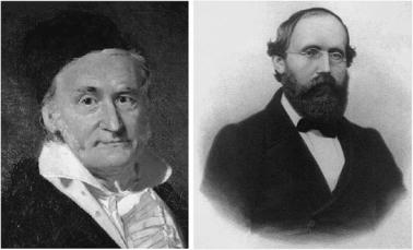
Fig. 3.2 Carl Friedrich Gauss (1777–1855) on the left and Georg Friedrich Bernhard Riemann (1826–1866) on the right. Gauss, the King of Mathematicians, was Professor at the University of Göttingen for many decades up to the very end of his long life. His contributions to all fields of Mathematics were enormous and most profound. Bernhard Riemann, another genious and a giant of human thought, had a very short and not too happy life. He was Gauss’ student both at the level of Diploma and of Habilitationsschrift. The whole of his work is contained in no more than 11 papers for a total of little more than 200 pages. Yet each of his contributions was a milestone in Mathematics and set the path for century long future developments. The foundations of Riemannian geometry were laid in the 16 page long dissertation of his Habilitation. Riemann had important ties with the Scuola Normale di Pisa and died in Italy at the age of 39

points in A and B, lying on the unique straight line which goes through any such pair of distinct points.

Curved surfaces were obviously known before Gauss, yet their shape and properties were conceived only through their immersion in three-dimensional space, considered unique and absolute, as pretended by Immanuel Kant who promoted Euclidian geometry to an a priori truth lying at the basis of any sensorial experience. Gauss revolutionary starting point was that of reformulating the geometrical study of surfaces from an intrinsic rather than extrinsic viewpoint. He wondered how a little being, confined to live on the surface, might have perceived the geometry of his world. Rather than viewing the global shape of the surface M, unaccessible to his observations, the little creature would have explored its local properties in the vicinity of a point p M.

In order to study curved surfaces in these terms, Gauss understood that it was necessary to abandon Cartesian coordinates as a system of point identification. In analytic geometry every point p E ≡ R3 of Euclidian space is singled out by a triplet of real numbers X, Y , Z which determine the distance of p from the three coordinate axes. As long as the points of the surface M are particular points of E, they admit the labeling in terms of three Cartesian coordinates, yet in such a description there is an excess of superfluous information. Why three coordinates when we are talking about a two-dimensional surface? Two should suffice. Gauss

Fig. 3.3 The points p of a curved surface M can be labeled with the three Cartesian coordinates X, Y, Z of the Euclidian space in which M is immersed. Yet this is a redundant information. The two Gaussian coordinates u and v are given through the construction of two systems of curves U and V on the surface

was the first to grasp the notion of curvilinear coordinates and invented Gaussian coordinates. A very simple but revolutionary idea.

On the surface M let us consider a family of curves U such that each element of the family never intersects any other element of the same family, at least in the neighborhood Up of the point p (for instance the lighter curves in Fig. 3.3) and such that the family covers the entire considered neighborhood. Let us next introduce a second family of curves V , with the same properties among themselves, yet such that each element of the family V intersects all elements of the U family at least in the neighborhood Up (for instance the darker curves Fig. 3.3). Once such systems of curves have been constructed, any point q Up in the neighborhood of p can be localized by stating on which U -curve and on which V -curve it lies. Assuming that u and v are the real parameters respectively enumerating the U and V curves, the pair of real numbers (u, v) provides the new (Gaussian) system of coordinates to label surface points. Using these coordinates we no longer need to make any reference to the exterior space in which M is immersed that might also be nonexisting!

By introducing curvilinear Gaussian coordinates the King of Mathematicians freed the study of surfaces from their immersion in the external Euclidian space E but he immediately had to cope with a new fundamental problem. Having abolished from the list of one’s mathematical instruments the straight line segments that join any two points A and B of the surface M, how can we calculate their distance? The great intuitions of Gauss were the tangent plane TpM and the linear element ds2, namely the metric.

Defining the absolute distance between two points A and B was no longer possible but also not interesting. In the external Euclidian space, the distance between A and B is the length of the segment which joins them, but which relevance has this datum for the little creature confined to live on the surface M, if such a segment does not lie on it? For the little two-dimensional being the only interesting datum is

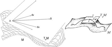
Fig. 3.4 The tangent plane to a point p of a surface M is a two-dimensional Euclidian space E2 where the notion of distance is defined. In the tangent plane which approximates infinitesimal regions of the surface surrounding p, we can define the line element as the Euclidian distance between two infinitesimally close points of the surface

the length of a road going from A to B: the length of any possible road with such a property! The small ant has exactly the same needs as any contemporary car-driver who wants to start on a journey. Both need to know the length of all possible paths from their origin to their destination.

Hence the problem addressed by Gauss was to give an answer to the following question: Can we define the length of any curve departing from p M and arriving at q M in terms of data completely intrinsic to the surface M?

Gauss’ answer was positive and based on the change of perspective at the basis of the new differential geometry.

Let us reformulate the initial question whether we might define the absolute distance between two arbitrary points A, B M of the surface, adding the extra condition that A and B should be only infinitesimally apart from each other. Analytically this means that if the Gaussian coordinates of A are (u, v), then those of B should be (u + du, v + dv) where du and dv are infinitesimal. Gauss crucial observation is that a very small portion of the surface M around any point p M can be approximated by a portion of the tangent plane to the surface at the point p, namely Tp M. Smaller the considered region of M better the approximation (see Fig. 3.4). This being the case we observe that Euclidian geometry makes sense in the tangent plane. Gauss remarked that the distance of two infinitesimally close points can be defined as the length of the infinitesimally short segment which joins them and which lies in the tangent plane.

Recalling Pithagora’s theorem one might be tempted to say that the square length of the segments joining A and B, named ds2, is the sum of the squared differences of the Gaussian coordinates, namely: ds2 = du2 + dv2. Yet this is not necessarily true. In order to apply Pithagora’s theorem it is required that the axes u and v be orthogonal, which is generically false. Indeed a priori it is by no means guaranteed that the curve u and the curve v, meeting at point A, should intersect there at right angle. In order to calculate ds2 one has therefore to find the components dx and

dy of the infinitesimal segment AB in an orthogonal system of axes x and y. Once

with matrix coefficients that vary from place to place on the surface, namely are functions of the Gaussian coordinate u, v. Taking this into account Gauss wrote the line element in the following way:

where F = a2 + c2, G = b2 + d2, H = 2ab + 2cd.

Formula (3.2.2), written in 1828 provided the first example (a two-dimensional one) of a Riemannian metric, although Riemann was at that time only a two-year old child.

3.2.2Bernhard Riemann Introduces n-Dimensional Metric

Manifolds

The name of Riemann is associated in Mathematics with so many different and fundamental objects that the contemporary student is instinctively led to think about the scientific production of this giant of human thought as composed by a countless number of papers, books and contributions. Actually the entire corpus of Riemann’s works is constituted only by 225 pages distributed over 11 articles published during the life-time of their author to which one has to add the 102 pages of the 4 posthumous publications. Among the latter there are the 16 pages of the Ueber die Hypothesen, welche der Geometrie zu Grunde liegen [2] which, in 1854, was debated by the candidate in front the Göttingen Faculty of Philosophy as Habilitationsschrift. The habilitation to teach courses was the traditional first step in the academic career foreseen by most European universities all over their very long history. In XIXth century Germany the procedure to access habilitation consisted of the writing of a dissertation on a topic chosen by the Faculty from a list of three proposed by the candidate. Typical time allowed for the preparation of such a dissertation was a couple of months and in the case of Riemann it amounted to exactly seven weeks.

Obsessed the whole of his short life by extreme poverty and by a very poor health that eventually led him to death from pulmonary consumption at the quite young age of thirty-nine, the shy and meek Bernhard Riemann, who was nonetheless quite conscious of his own talents, had already profoundly impressed Gauss with his diploma thesis. Written in 1851 and entitled Grundlagen für eine allgemeine Theorie der Functionen einer veränderlichen complexen Grösse which can be translated as Principles of a General Theory of the Functions of one complex

of different measure-relations, and consequently that space is only a particular case of a triply extended magnitude.

In contemporary language the multiply extended magnitudes2 were simply the manifolds which we discussed in Chap. 2 and the measure relations are just the metric to be discussed in the present chapter and introduced for the first time by Gauss through (3.2.2).

Following the new road opened by Gauss with the Disquisitiones, Riemann introduced n-extended manifolds whose points are labeled by n rather than two curvilinear coordinates xi and introduced the line element as a generic symmetric quadratic form in the differentials of these coordinates:

The coefficients of this quadratic form gij (x) were later known as the Riemannian metric tensor.

Riemann grasped the main point, namely that the geometry of manifolds is encoded in the possible metric tensors or measure relations, as he called them, and made the following bold statement: Hence flows as a necessary consequence that the propositions of geometry cannot be derived from general notions of magnitude, but that the properties which distinguish space from other conceivable triply extended magnitudes are only to be deduced from experience. Thus arises the problem, to discover the simplest matters of fact from which the measure-relations of space may be determined; a problem which from the nature of the case is not completely determinate, since there may be several systems of matters of fact which suffice to determine the measure-relations of space.

In other words, the young genius was aware that the same manifold could support quite different metrics and thought that this applied in particular to Space, i.e. to the 3-dimensional physical world of our sensorial experience. He posed himself the question which should be the metric of Space and came to the conclusion that such a question could only be answered through experiment. This amounted to say that the geometry of the world is a matter of Physics and not of a priori Philosophy or Mathematics. Such a sentence of Riemann must have influenced Einstein quite deeply. Indeed the final outcome of Einstein Theory of Relativity is that the geometry of space-time is dynamically determined by its matter content through Einstein field equations.

In considering such a question as what is the preferred metric to be selected for a given manifold, Riemann formulated the basic problem of invariants. The matter of facts3 to which he alluded are the intrinsic properties encoded in a given metric tensor namely its invariants and he formulated the problem of determining, for instance, the minimal complete number of invariants able to select Euclidian geometry. In his quest for these invariants he came to the notion of the Riemann

2In the original German text of Riemann these were named mehrfach ausgedehnter Grossen. In modern scientific German the notion of manifolds is referred to as mannigfaltigkeiten.

3Einfachsten Thatsachen in the original German text.