6.3 Interior Solutions and the Stellar Equilibrium Equation

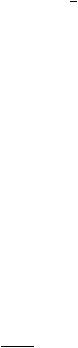
Fig. 6.4 The fluid composing the static star must be at rest on the space-like surfaces t = const. Hence the world-lines of the fluid elements must admit the Killing vector field ξ ≡ ∂∂t as tangent vector

Correspondingly the flat intrinsic components T ab ≡ Vμa VνbT μν of the stress-energy tensor are simply given by:

The intrinsic components of the Einstein tensor for the spherical symmetric static metric (6.3.1) have already been calculated in (5.9.15). Introducing the convenient definitions:

Combining (6.3.10) with (6.3.8) we see that Einstein equations reduce, in this case, to a system of three ordinary differential equations for the four functions h(r), f (r), p(r), ρ(r). This is undetermined if we do not specify the nature of the fluid we are considering by writing an equation of state, namely a relation between the pressure and the energy density:

The function F appearing in (6.3.11) encodes all the thermodynamical properties of the fluid.

Consider the equation:

by a straightforward integration we obtain:

If we have a spherical distribution of mass-energy the integral:

is immediately interpreted as the total mass-energy contained in a sphere of radius R. Hence solving (6.3.13) with respect to the function h(R) we obtain:

which still contains the undetermined integration constant introduced in (6.3.13). This latter is fixed imposing the boundary condition h(0) = 1 that corresponds to the regularity of space-time in the origin. In this way we conclude that:

Equation (6.3.16) shows that the radial-radial component of the metric has, in presence of spherically distributed matter, the same form as in the case of the Schwarzschild vacuum metric. The only difference resides in that the constant parameter m of the Schwarzschild metric (4.3.1) is replaced by the function M(R) introduced in (6.3.14) and representing the total mass contained in a sphere of radius R. At this point a subtle remark on M(R) is in order. Its explicit form has emerged from the integration of one of the Einstein equations and we interpreted it as the total mass contained in a sphere of radius R. To be very precise such an interpretation is illegal since it uses the integration measure of flat space rather than the integration measure determined by the true space-time metric. Given the mass

248 6 Stellar Equilibrium

density ρ(x), the proper mass contained in a sphere of radius R is actually defined by the integral:

where g3 is the metric of a 3-dimensional section of space-time at constant time. Having found the solution (6.3.16) we actually have:

(6.3.18) In other words the proper mass contained in a sphere of radius R is strictly larger than the effective mass contained in the same sphere and determining the metric through Einstein equation. This is not a discrepancy rather it encodes a profound physical fact. Indeed the difference:

Mp (R) − M(R)

has a clearcut meaning, it is the gravitational binding energy. Just as the mass of a Helium nucleus is smaller than the sum of the masses of two protons and two neutrons in the same way the mass of a star is smaller than the sum of the masses of all its components.

Having cleared the meaning of M(R) we come back to the Einstein equations following from the explicit form of the Einstein tensor (6.3.10). So far we have solved only one of them, namely (6.3.12), which has determined the form of the radial-radial component of the metric h(r). Next equation to be considered is:

which allows for the determination of the time-time component f (r) = exp[2a(r)]. From (6.3.19) we obtain:

Equation (6.3.21) determines a(r) and hence f (r) by means of a simple integration in r:

It is interesting to appreciate the physical meaning of (6.3.21) by considering its non-relativistic approximation. On one side we recall that:

where V (r) is the gravitational potential. On the other hand the non-relativistic approximation corresponds to the regime where we have:

These conditions (6.3.24) are easily explained as follows. First of all let us recall that a non-relativistic regime is obtained when:

which is easily seen to be true if one recalls the equation of state of ideal gases pV = nRT and that temperature measures the average kinetic energy per degree of freedom. On the other hand M(r)c2 is the rest energy contained in a sphere of radius r. Therefore in natural units where c = G = 1 the first of (6.3.24) is just the statement (6.3.25). The second condition (6.3.24) is instead the statement that the Schwarzschild radius of the total mass contained in a sphere of radius r is much smaller than the radius r itself. Indeed such a Schwarzschild radius is rS (r) = 2 cG2 M(r) and, in natural units, the second of conditions (6.3.24) states that rS (r) r. Inserting the non-relativistic approximations (6.3.23) and (6.3.24) into (6.3.21) we find:

which is the correct differential equation for the Newtonian potential generated by a spherical mass distribution.

Having dealt with the equations associated with the first and second independent components of the Einstein tensor (see (6.3.10)) we have determined the two unknown coefficients of the metric in terms of the radial mass-distribution ρ(r). We still have to determine the radial behavior of the pressure p(r) related to the radial mass-distribution ρ(r) by the equation of state (6.3.11). This information is encoded in the third and fourth Einstein equations:

Since Einstein equations are not independent being related by the Bianchi identity that implies the covariant conservation of the stress-energy tensor, an alternative