

170 |
4 Motion in the Schwarzschild Field |
of lengths and the non-relativistic regime is approached when the actual orbit radius r is big with respect to m. Hence the post-Newtonian development corresponds to a series expansion in the dimensionless parameter:
|
|
|
|
|
|
|
|
|
|
|
|
m |
1 |
|
|
|
|
|
|
|
|
(4.3.36) |
|||||
|
|
|
|
|
|
|
|
|
|
|
|
|
|
|
|
|
|
|
|
|
|
|
|
||||
|
|
|
|
|
|
|
|
|
|
|
|
|
r |
|
|
|
|
|
|
|
|
||||||
Hence we can write: |
|
|
|
|
|
|
|
|
|
|
|
|
|
|
|
|
|
|
|
|
|
|
|
|
|
|
|
E (r) |
= |
|
|
1 − 2 mr |
|
|
1 |
− |
2 |
m |
1 |
+ |
3 m |
|
(4.3.37) |
||||||||||||
|
|
|
|
|
|
|
|
|
|
|
|
|
|
||||||||||||||
|
1 − 3 mr |
|
|
|
|
|
|
r |
2 r |
+ · · · |
|
||||||||||||||||
|
|
1 |
− |
1 m |
+ |
O |
m2 |
|
|
|
|
|
|
|
|
|
(4.3.38) |
||||||||||
|
|
|
|
|
|
|
|
|
|
|
|
|
|
||||||||||||||
|
2 r |
|
|
|
|
|
|
|
|
|
|||||||||||||||||
|
|
|
|
|
|
r2 |
|
|
|
|
|
|
|
|
|
|
|
||||||||||
and comparing (4.3.38) with (4.3.15) we obtain:
5 |
|
E |
|
|
|
E |
|
1 m |
|
||||
E = |
1 + 2 |
|
|
|
1 + |
|
+ · · · 1 − |
|
|
|
+ · · · |
||
μc2 |
μc2 |
2 r |
|||||||||||
|
E = − |
1 GMμ |
|
|
|
|
|
(4.3.39) |
|||||
|
|
|
|
|
|
|
|
|
|
||||
2 |
|
r |
|
|
|
|
|
||||||
The last line in (4.3.39) correctly reproduces the Newtonian result for the energy of a particle of mass μ bounded on a circular orbit around a center of mass M. Indeed if we consider the effective Newtonian potential:
Veff(Newton) |
= |
1 |
2 |
− |
GMμ |
(4.3.40) |
|||
2 |
|
μr2 |
r |
||||||
and we calculate its minimum: |
|
|
|
|
|
|
|
|
|
∂V |
(Newton) |
|
|
||||||
|
|
eff |
|
|
|
= 0 |
|
(4.3.41) |
|
|
|
|
|
|
|
||||
∂r
we obtain the condition of balance between the centrifugal energy and the potential energy:
2 |
= |
GMμ |
(4.3.42) |
μr2 |
r |
which inserted in the Newtonian formula (4.2.1) for the particle energy, together with the circular orbit condition (r˙) gives back (4.3.39).
4.4 The Periastron Advance of Planets or Stars
Let us now go back to (4.3.10) and to the second of (4.3.6) that are the exact relativistic definitions of energy and angular momentum in Schwarzschild geometry.

4.4 The Periastron Advance |
171 |
Making a substitution similar to the substitution (4.2.3) used in the Newtonian case, namely:
|
dr |
; |
|
r |
|
|
dr |
; |
|
˙ = |
r |
r |
|
||
˙ ≡ dτ |
|
≡ dφ |
|
|
|||||||||||
r |
|
|
|
|
|
|
|
|
|
r |
L |
(4.4.1) |
|||
|
|
|
|
|
|
|
|
|
2 |
||||||
(4.3.10) becomes: |
|
|
|
|
|
|
|
|
|
|
|
|
|
|
|
u 2 + u2 = C0 + 2C1u + |
2 |
C2u3 |
|
(4.4.2) |
|||||||||||
|
|
||||||||||||||
3 |
|
||||||||||||||
where: |
|
|
|
|
|
|
|
|
|
|
|
|
|
|
|
|
|
C |
0 |
= |
E 2 − 1 |
= |
2Eμ |
|
|
(4.4.3) |
|||||
|
|
|
|
2 |
|
|
|
|
|||||||
|
|
|
L2 |
|
|
|
|
|
|
||||||
|
|
|
|
|
m |
GMμ2 |
|
|
|
|
|
||||
|
|
C1 = |
|
= |
|
2 |
|
|
|
|
(4.4.4) |
||||
|
|
L2 |
|
|
|
|
|
||||||||
|
|
C2 = 3m |
|
|
|
|
|
|
|
(4.4.5) |
|||||
The definition (4.4.3), (4.4.4) of the parameters C0,1 is consistent with their previous Newtonian definition (4.2.7) thanks to the relation (4.3.15) between the relativistic first integrals E , L and their Newtonian analogues E, . Equation (4.4.2) is the differential orbit equation in Schwarzschild geometry and replaces the Newtonian equation (4.2.6): the difference resides in the term cubic in u with coefficient C2 = 2m. In full analogy with the procedure followed in the Newtonian case we take a further derivative of (4.4.2) and we obtain:
2u u + u − C1 − C2u2 = 0 |
(4.4.6) |
which admits two kinds of solutions, the already discussed circular orbits (u = 0) and the non-circular ones that satisfy the differential equation:
u + u − C1 = C2u2 |
(4.4.7) |
replacing the Keplerian equation (4.2.9).
In the limit where C2u2 is negligible with respect to the other terms the general solution of (4.4.7) becomes (4.2.11) which, as we know, describes an elliptic orbit of semilatus rectum a and eccentricity e, the constant C1 being:
1 |
|
C1 = a(1 − e2) |
(4.4.8) |
We can appreciate the difference between General Relativity and Newtonian physics if we study numerical solutions of (4.4.7) with the help of a computer programme. To this effect it is convenient to measure the radius r and the semilatus
rectum a in units of the Schwarzschild emiradius m by setting |
|
|
u = u ; |
a = am |
(4.4.9) |
m

172 |
4 Motion in the Schwarzschild Field |
Fig. 4.9 Schwarzschild geometry: Orbit of a massive test particle with Keplerian parameters a = 70m and
e = 0.7 after 1 revolution
which, combined with (4.4.8), (4.4.5) reduces (4.4.7) to the form:
|
+ |
|
− |
|
|
1 |
|
= 3 |
|
2 |
(4.4.10) |
u |
u |
|
|
|
|
u |
|||||
a(1 |
− |
e2) |
|||||||||
|
|
|
|
|
|
|
|
|
|
|
|
Equation (4.4.10) is of the second order and numerical solutions can be obtained if we feed the computer programme with two initial conditions. The initial conditions appropriate to describe the physical problem we investigate are the following ones:
|
|
|
|
|
|
1 |
|
(4.4.11) |
|
u(0) = |
|
|
|
|
|||
|
a(1 |
− |
e) |
|||||
|
|
|
|
|
|
|
|
|
|
|
(0) = 0 |
|
(4.4.12) |
||||
u |
|
|
||||||
Equation (4.4.12) fixes the origin of the φ angle at the periastron namely at the point in the orbit where the derivative of the radius goes to zero. Equation (4.4.12) states that distance of the test particle from the star at the first periastron is the same as it would be in a Keplerian orbit, namely r− = a(1 − e) (compare with Fig. 4.4). Given the initial conditions the subsequent n revolutions of the test particle are numerically determined by the differential equation. It is clear from our previous discussions that the relativistic effects will be evident only in narrow systems where a is small and in eccentric orbits e → 1. So in order to emphasize the size of these effects we have chosen an example with the following parameters:
|
= 70; e = 0.7 |
(4.4.13) |
a |
In Fig. 4.9 we display the shape of the orbit for this system after one revolution. As it can be visually appreciated the orbit is nearly an ellipsis but not quite. At φ = 2π the test particle is at a distance r(2π ) close to the initial value r(0) but slightly bigger. Furthermore the second periastron, namely the angle φ1 corresponding to the second zero of the derivative r is not exactly at φ1 = 2π but at a slightly earlier angle φ1 = 2π − Δφ. The phenomenon is more clearly understood if we allow the computer programme to run for more revolutions. Figure 4.10 displays three revolutions of the same physical system. At each revolution the periastron is anticipated of some
4.4 The Periastron Advance |
173 |
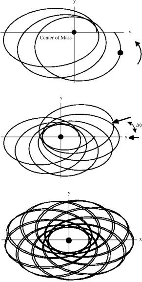
Fig. 4.10 Schwarzschild geometry: Orbit of a massive test particle with Keplerian parameters a = 70m and
e = 0.7 after 3 revolution
Fig. 4.11 Schwarzschild geometry: Orbit of a massive test particle with Keplerian parameters a = 70m and
e = 0.7 after 7 revolution
Fig. 4.12 Schwarzschild geometry: Orbit of a massive test particle with Keplerian parameters a = 70m and
e = 0.7 after 20 revolution
angle Δφ with respect to 2π . This is further stressed by Fig. 4.11 that shows the orbit after 7 revolutions.
It is interesting to understand which kind of pattern emerges at asymptotically late times after many revolutions. This is revealed by looking at Fig. 4.12 which shows the orbit after 20 revolutions. What we witness is a sort of symmetry restoration mechanism. In Newtonian physics the eccentric orbits break the spherical symmetry of the Hamiltonian. In general relativity, due to the periastron advance the