

162 |
|
|
|
|
|
|
|
4 Motion in the Schwarzschild Field |
|
2 |
r+ −r− |
|
|
|
|
|
|
|
|
eccentricity e |
, r |
± |
|
|
|
|
|
|
|
|
= r+ +r− |
|
|
|
|
|
|
|
|
being the maximal and |
|
|
|
|
|
|
|
||
minimal distances from the |
|
|
|
|
|
|
|||
center of mass reached by the |
|
|
|
|
|
|
|||
test particle while going |
|
|
|
|
|
|
|
||
around its orbit. In the case of |
|
|
|
|
|
|
|||
the Solar system these points |
|
|
|
|
|
|
|||
are respectively named the |
|
|
|
|
|
|
|||
aphelion and the perihelion |
|
|
|
|
|
|
|||
|
|
|
1 |
= r |
= a 1 − e2 |
1 |
|
e1cos φ |
(4.2.11) |
|
|
|
u |
+ |
|||||
where we named: |
|
|
|
|
|
|
|
||
|
|
|
|
|
|
|
|
||
|
|
|
C1 |
≡ a = semilatus rectum |
|
||||
|
|
|
1 − e2 |
(4.2.12) |
|||||
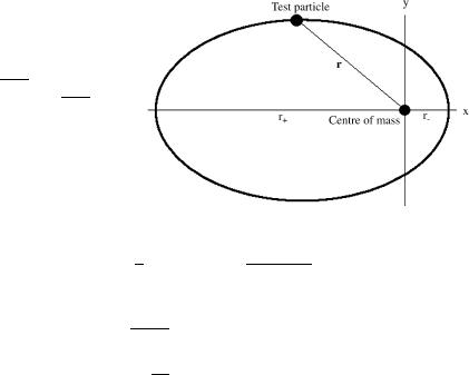
Fig. 4.4 The Keplerian orbit |
b |
≡ e = eccentricity |
|
||||||
C1 |
|
||||||||
of a test particle of mass μ |
|
|
|
|
|
|
|||
around a center of mass M is an ellipsis parameterized by
the semilatus rectum a = r+ +r− and the
In this way the parameter e, whose range is 0 ≤ e ≤ 1, replaces the integration constant b while the second integration constant φ0 is reabsorbed into the definition of the azimuthal angle φ. The names given to the parameters (4.2.12) are traditional in astronomy since the time of Kepler and refer to the geometrical interpretation of the solution (4.2.11) as the equation of an ellipsis (see Fig. 4.4). The geometrical parameters a and e are related to the physical constants of motion, namely to the energy E and the angular momentum .
4.3The Orbit Equations of a Massive Particle in Schwarzschild Geometry
Let us now turn to the description of space-time as a differentiable manifold endowed with a pseudo-Riemannian structure and introduce the Schwarzschild (see Fig. 4.5) metric [1]:
ds2 |
1 |
− |
2 |
m |
dt2 |
1 |
− |
2 |
m |
−1dr2 |
+ |
r2 |
dθ 2 |
+ |
sin2 |
θ dφ2 |
(4.3.1) |
|
|
||||||||||||||||
|
= − |
|
r |
+ |
|
r |
|
|
|
|
|
||||||
where t denotes the time coordinates, while r, θ , φ are polar coordinates in the same notations as before.
To obtain the geodesic equation for the motion of a massive test particle in the metric (4.3.1) we use the variational principle. As we explained in Sect. 3.8, given

4.3 The Orbit Equations of a Massive Particle |
163 |
Fig. 4.5 Karl Schwarzschild (1873–1916) was born in Frankfurt am Mein from a well-to-do Jewish family. He published his first papers in astronomy when he was still a boy. In 1889–1890 he published two articles on the determination of orbits for binary stars. Next year he obtained his doctorate in Astronomy from the University of Munich. After an experience at the observatories of Vienna and Munich, in 1900 he was appointed Director of the Astronomical Observatory of Göttingen where he interacted with such personalities as David Hilbert and Hermann Minkowski. In 1909 he moved to the Observatory of Postdam. By this time he was already a famous scientist, member of the Prussian Academy of Sciences since 1912. His contributions concerned various fields of physics related with Astronomy. In particular he studied the equilibrium equations of radiation and was the first to discover radiation pressure. At the breaking of World War I in 1914, notwithstanding his forty years of age he enrolled in the German Army and fought first on the Western Front in Belgium, then on the Eastern Front in Russia. In 1916, while at the front, he wrote two scientific articles. One less famous than the second contains quantization rules similar to those of Bohr and Sommerfeld, discovered by him independently. The second article contains the Schwarzschild solution of Einstein equations. He had learnt of Einstein new theory of General Relativity just a couple of months before reading the issue 25 of the Proceedings of the Prussian Academy of Sciences of November 1915. His simple and elegant solution of Einstein field equations was sent to Einstein that answered to him with the following words: have read your paper with the utmost interest. I had not expected that one could formulate the exact solution of the problem in such a simple way. I liked very much your mathematical treatment of the subject. Next Thursday I shall present the work to the Academy with a few words of explanation. The same year, 1916, Schwarzschild died from a rare skin infection contracted on the war front
an explicit metric gμν (x) we have the proper time functional of (3.8.6) and (3.8.7) which leads to Euler-Lagrange equations plus the auxiliary condition 2L = 1. Following this reasoning, from the Schwarzschild metric (4.3.1) we derive the effective Lagrangian:
− |
L |
1 |
− |
2 |
m |
t2 |
1 |
− |
2 |
m |
−1r2 |
+ |
r2 |
θ |
2 |
+ |
sin2 θ φ2 |
(4.3.2) |
r |
r |
|
||||||||||||||||
|
= − |
|
˙ + |
|
|
˙ |
|
˙ |
|
˙ |
|
where the dot denotes the derivative d/dτ with respect to proper time. The Euler-Lagrange equation of the field θ (τ ) yields:

164 |
4 Motion in the Schwarzschild Field |
|
|
|
|
|
|
d |
|
∂L |
− |
∂L |
= 0 |
|
||
|
|
|
|
|
dτ |
|
θ |
∂θ |
|
|||||
d |
− |
2r |
2 |
˙ + |
|
|
∂ ˙ |
|
˙ |
2 |
= |
0 |
|
|
|
|
|
|
|
||||||||||
dτ |
|
|
|
|
|
|||||||||
|
|
|
θ |
|
2 sin θ cos θ φ |
|
|
|
||||||
From 4.3.3 we conclude that it is consistent to set:
θ = const = π 2
(4.3.3)
(4.3.4)
throughout the motion. In other words the Schwarzschild motion is planar as the Newtonian motion: it takes place in the equatorial plane with respect to the coordinate frame we have adopted (see Fig. 4.3). Taking this into account we immediately get the following reduced Lagrangian:
L reduc. |
= |
1 |
|
1 |
− |
2 |
m |
t2 |
1 |
− |
2 m |
−1r2 |
+ |
r |
2φ2 |
|
(4.3.5) |
|
2 |
r |
|||||||||||||||||
|
|
− |
|
˙ + |
|
r |
˙ |
|
˙ |
|
|
It is apparent from (4.3.5) that both the time t and the azimuthal angle φ are cyclic canonical variables, namely they appear in the Lagrangian only through their derivatives with respect to the Lagrangian time τ . This implies the existence of two first integrals of the motion, namely:
|
|
|
dτ |
− |
r |
|
= |
|
= |
|
|||
t-variation |
|
|
dt |
1 |
|
2 m |
|
|
E |
|
const |
||
|
|
|
|
|
|
|
|||||||
|
|
|
|
dφ |
|
|
|
|
|
|
(4.3.6) |
||
φ-variation |
r2 |
= L = const |
|
|
|||||||||
|
|
|
|
||||||||||
dτ |
|
|
|||||||||||
It is tempting to interpret E and L as the energy and the angular momentum, respectively. Comparison with the Newtonian theory will confirm such an interpretation.
Since 2L = 1 along the geodesics, rather than working out the additional EulerLagrange equation (for the r-variation) we just insert (4.3.6) into (4.3.5) and we get:
1 |
= |
|
|
E 2 |
|
|
|
r˙2 |
|
|
|
|
r2 |
L2 |
(4.3.7) |
|||||
1 |
|
2 m − |
1 |
|
|
|
|
|
|
|
r4 |
|||||||||
|
− |
− |
2 m − |
|
|
|
||||||||||||||
|
|
|
|
r |
|
|
|
r |
|
|
|
|
|
|
|
|
||||
so that we obtain: |
|
|
|
|
|
|
|
|
|
|
|
|
|
|
|
|
|
|
|
|
|
|
|
dr |
2 |
|
Veff (r) |
= |
E 2 |
|
|
||||||||||
|
|
dτ |
|
|
|
|||||||||||||||
|
|
|
|
+ |
|
|
|
|
|
|
|
|
|
|
|
(4.3.8) |
||||
|
|
|
|
|
|
|
|
|
|
dφ |
|
|
|
L |
|
|||||
|
|
|
|
|
|
|
|
|
|
= |
|
|
||||||||
|
|
|
|
|
|
|
|
|
|
|
|
|
|
|
|
|||||
|
|
|
|
|
|
|
|
|
|
dτ |
r2 |
|
|
|||||||
where we have introduced the following effective central potential:
Veff |
≡ |
1 |
− |
2 |
m |
1 |
|
|
L2 |
|
|
|
||
|
|
|
|
|
||||||||||
|
|
|
|
r |
+ r2 |
|
||||||||
|
|
|
|
m |
|
L2 |
|
|
|
L2m |
|
|||
|
= |
1 − 2 |
|
+ r2 |
− |
2 |
|
|
(4.3.9) |
|||||
|
r |
r3 |
|
|||||||||||