

- •Preface
- •Acknowledgements
- •Contents
- •1.1 Introduction
- •1.2 Classical Physics Between the End of the XIX and the Dawn of the XX Century
- •1.2.1 Maxwell Equations
- •1.2.2 Luminiferous Aether and the Michelson Morley Experiment
- •1.2.3 Maxwell Equations and Lorentz Transformations
- •1.3 The Principle of Special Relativity
- •1.3.1 Minkowski Space
- •1.4 Mathematical Definition of the Lorentz Group
- •1.4.1 The Lorentz Lie Algebra and Its Generators
- •1.4.2 Retrieving Special Lorentz Transformations
- •1.5 Representations of the Lorentz Group
- •1.5.1 The Fundamental Spinor Representation
- •1.6 Lorentz Covariant Field Theories and the Little Group
- •1.8 Criticism of Special Relativity: Opening the Road to General Relativity
- •References
- •2.1 Introduction
- •2.2 Differentiable Manifolds
- •2.2.1 Homeomorphisms and the Definition of Manifolds
- •2.2.2 Functions on Manifolds
- •2.2.3 Germs of Smooth Functions
- •2.3 Tangent and Cotangent Spaces
- •2.4 Fibre Bundles
- •2.5 Tangent and Cotangent Bundles
- •2.5.1 Sections of a Bundle
- •2.5.2 The Lie Algebra of Vector Fields
- •2.5.3 The Cotangent Bundle and Differential Forms
- •2.5.4 Differential k-Forms
- •2.5.4.1 Exterior Forms
- •2.5.4.2 Exterior Differential Forms
- •2.6 Homotopy, Homology and Cohomology
- •2.6.1 Homotopy
- •2.6.2 Homology
- •2.6.3 Homology and Cohomology Groups: General Construction
- •2.6.4 Relation Between Homotopy and Homology
- •References
- •3.1 Introduction
- •3.2 A Historical Outline
- •3.2.1 Gauss Introduces Intrinsic Geometry and Curvilinear Coordinates
- •3.2.3 Parallel Transport and Connections
- •3.2.4 The Metric Connection and Tensor Calculus from Christoffel to Einstein, via Ricci and Levi Civita
- •3.2.5 Mobiles Frames from Frenet and Serret to Cartan
- •3.3 Connections on Principal Bundles: The Mathematical Definition
- •3.3.1 Mathematical Preliminaries on Lie Groups
- •3.3.1.1 Left-/Right-Invariant Vector Fields
- •3.3.1.2 Maurer-Cartan Forms on Lie Group Manifolds
- •3.3.1.3 Maurer Cartan Equations
- •3.3.2 Ehresmann Connections on a Principle Fibre Bundle
- •3.3.2.1 The Connection One-Form
- •Gauge Transformations
- •Horizontal Vector Fields and Covariant Derivatives
- •3.4 Connections on a Vector Bundle
- •3.5 An Illustrative Example of Fibre-Bundle and Connection
- •3.5.1 The Magnetic Monopole and the Hopf Fibration of S3
- •The U(1)-Connection of the Dirac Magnetic Monopole
- •3.6.1 Signatures
- •3.7 The Levi Civita Connection
- •3.7.1 Affine Connections
- •3.7.2 Curvature and Torsion of an Affine Connection
- •Torsion and Torsionless Connections
- •The Levi Civita Metric Connection
- •3.8 Geodesics
- •3.9 Geodesics in Lorentzian and Riemannian Manifolds: Two Simple Examples
- •3.9.1 The Lorentzian Example of dS2
- •3.9.1.1 Null Geodesics
- •3.9.1.2 Time-Like Geodesics
- •3.9.1.3 Space-Like Geodesics
- •References
- •4.1 Introduction
- •4.2 Keplerian Motions in Newtonian Mechanics
- •4.3 The Orbit Equations of a Massive Particle in Schwarzschild Geometry
- •4.3.1 Extrema of the Effective Potential and Circular Orbits
- •Minimum and Maximum
- •Energy of a Particle in a Circular Orbit
- •4.4 The Periastron Advance of Planets or Stars
- •4.4.1 Perturbative Treatment of the Periastron Advance
- •References
- •5.1 Introduction
- •5.2 Locally Inertial Frames and the Vielbein Formalism
- •5.2.1 The Vielbein
- •5.2.2 The Spin-Connection
- •5.2.3 The Poincaré Bundle
- •5.3 The Structure of Classical Electrodynamics and Yang-Mills Theories
- •5.3.1 Hodge Duality
- •5.3.2 Geometrical Rewriting of the Gauge Action
- •5.3.3 Yang-Mills Theory in Vielbein Formalism
- •5.4 Soldering of the Lorentz Bundle to the Tangent Bundle
- •5.4.1 Gravitational Coupling of Spinorial Fields
- •5.5 Einstein Field Equations
- •5.6 The Action of Gravity
- •5.6.1 Torsion Equation
- •5.6.1.1 Torsionful Connections
- •The Torsion of Dirac Fields
- •Dilaton Torsion
- •5.6.2 The Einstein Equation
- •5.6.4 Examples of Stress-Energy-Tensors
- •The Stress-Energy Tensor of the Yang-Mills Field
- •The Stress-Energy Tensor of a Scalar Field
- •5.7 Weak Field Limit of Einstein Equations
- •5.7.1 Gauge Fixing
- •5.7.2 The Spin of the Graviton
- •5.8 The Bottom-Up Approach, or Gravity à la Feynmann
- •5.9 Retrieving the Schwarzschild Metric from Einstein Equations
- •References
- •6.1 Introduction and Historical Outline
- •6.2 The Stress Energy Tensor of a Perfect Fluid
- •6.3 Interior Solutions and the Stellar Equilibrium Equation
- •6.3.1 Integration of the Pressure Equation in the Case of Uniform Density
- •6.3.1.1 Solution in the Newtonian Case
- •6.3.1.2 Integration of the Relativistic Pressure Equation
- •6.3.2 The Central Pressure of a Relativistic Star
- •6.4 The Chandrasekhar Mass-Limit
- •6.4.1.1 Idealized Models of White Dwarfs and Neutron Stars
- •White Dwarfs
- •Neutron Stars
- •6.4.2 The Equilibrium Equation
- •6.4.3 Polytropes and the Chandrasekhar Mass
- •6.5 Conclusive Remarks on Stellar Equilibrium
- •References
- •7.1 Introduction
- •7.1.1 The Idea of GW Detectors
- •7.1.2 The Arecibo Radio Telescope
- •7.1.2.1 Discovery of the Crab Pulsar
- •7.1.2.2 The 1974 Discovery of the Binary System PSR1913+16
- •7.1.3 The Coalescence of Binaries and the Interferometer Detectors
- •7.2 Green Functions
- •7.2.1 The Laplace Operator and Potential Theory
- •7.2.2 The Relativistic Propagators
- •7.2.2.1 The Retarded Potential
- •7.3 Emission of Gravitational Waves
- •7.3.1 The Stress Energy 3-Form of the Gravitational Field
- •7.3.2 Energy and Momentum of a Plane Gravitational Wave
- •7.3.2.1 Calculation of the Spin Connection
- •7.3.3 Multipolar Expansion of the Perturbation
- •7.3.3.1 Multipolar Expansion
- •7.3.4 Energy Loss by Quadrupole Radiation
- •7.3.4.1 Integration on Solid Angles
- •7.4 Quadruple Radiation from the Binary Pulsar System
- •7.4.1 Keplerian Parameters of a Binary Star System
- •7.4.2 Shrinking of the Orbit and Gravitational Waves
- •7.4.2.1 Calculation of the Moment of Inertia Tensor
- •7.4.3 The Fate of the Binary System
- •7.4.4 The Double Pulsar
- •7.5 Conclusive Remarks on Gravitational Waves
- •References
- •Appendix A: Spinors and Gamma Matrix Algebra
- •A.2 The Clifford Algebra
- •A.2.1 Even Dimensions
- •A.2.2 Odd Dimensions
- •A.3 The Charge Conjugation Matrix
- •A.4 Majorana, Weyl and Majorana-Weyl Spinors
- •Appendix B: Mathematica Packages
- •B.1 Periastropack
- •Programme
- •Main Programme Periastro
- •Subroutine Perihelkep
- •Subroutine Perihelgr
- •Examples
- •B.2 Metrigravpack
- •Metric Gravity
- •Routines: Metrigrav
- •Mainmetric
- •Metricresume
- •Routine Metrigrav
- •Calculation of the Ricci Tensor of the Reissner Nordstrom Metric Using Metrigrav
- •Index

250 |
6 Stellar Equilibrium |
and simpler way of determining the radial behavior of the pressure is provided by writing such a conservation law. In flat anholonomic indices we have:
cTabηcb = 0 |
|
|
(6.3.29) |
∂cTabηca + ωc|af Tgbηca ηf g + ωc|bf Tga ηca ηf g = 0 |
|
Using the particular structure of Tab and choosing for instance b = 1 we get: |
|
−∂1T11 − ωc|a1T11ηca + ωc|1f Tag ηca ηf g = 0 |
|
|
(6.3.30) |
−∂1T11 − (ω0|01 − ω2|21 − ω3|31)T11 = 0
Inserting the explicit form (5.9.5) of the spin connection for a spherically symmetric static metric, the non-vanishing components with an index 1 are:
|
|
ω0|01 = −a e−b |
|
||||
|
|
ω2|21 |
= − |
e−b |
(6.3.31) |
||
|
|
|
r |
||||
|
|
ω3|31 |
= − |
e−b |
|
||
|
|
|
r |
|
|||
while the intrinsic derivative ∂1 is defined by |
|
|
|
||||
|
|
∂1 ≡ e−b |
1 |
|
(6.3.32) |
||
|
|
|
|
||||
∂r |
|||||||
Inserting (6.3.32) and (6.3.31) into 6.3.30) we find: |
|
||||||
|
d |
|
|
|
|
|
|
− |
|
p(r) − a (p + ρ) = 0 |
(6.3.33) |
||||
dr |
|||||||
which combined with (6.3.21) yields the Tolman-Oppenheimer-Volkoff relativistic equation of stellar equilibrium:
d |
p(r) |
(p |
ρ) |
M(r) + |
4π r3p(r) |
(6.3.34) |
|
[ − |
] |
||||
dr |
= − + |
|
r r |
2M(r) |
|
|
6.3.1Integration of the Pressure Equation in the Case of Uniform Density
A very simple and idealized model of a star corresponds to choosing a uniform density:
ρ(r) = ρ0 = const |
(6.3.35) |
6.3 Interior Solutions and the Stellar Equilibrium Equation |
251 |
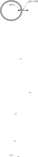
Fig. 6.5 The total force exerted by pressure on the spherical stratum of matter contained between the spherical surface of radius r and the spherical surface of radius r + dr is given by [p(r + dr) − p(r)] × 4π r2. On the other hand the gravitational force exerted on the same stratum of matter by the matter contained in the sphere of radius r is, by Newton’s law, −ρ0 × 4πρ0r2 × . Hence the equilibrium equation is obtained by balancing these two forces
In this case the function M(r) is immediately determined and we obtain:
M(r) = |
4 |
πρ0r3 |
(6.3.36) |
3 |
6.3.1.1 Solution in the Newtonian Case
If we consider the stellar equilibrium problem in the contest of Newtonian Physics, what we have to write is simply the following equation:
dp |
= −ρ0 |
M(r) |
= − |
4 |
πρ0r |
(6.3.37) |
dr |
r2 |
3 |
which expresses the balancing of the pressure repulsive force with the gravitational attractive force (see Fig. 6.5). Equation (6.3.37) is immediately integrated to give:
p(r) = − |
2 |
πρ02r2 + const |
(6.3.38) |
3 |
The integration constant is fixed by imposing the obvious boundary condition that the pressure should vanish where the star ends, namely p(R) = 0 if R is the radius of the spherical star. The solution of the differential equation with this boundary condition becomes:
p(r) = 2 πρ2 R2 − r2
3 0
If we denote the total mass of the star by
M ≡ 4 πρ0R3
3
then the Newtonian solution (6.3.39) can be rewritten as follows:
|
|
|
3 |
|
|
2 |
1 |
|
|
r |
|
p(r) |
= |
|
|
M |
− |
||||||
|
|
|
|
|
|||||||
|
8π R4 |
|
R |
||||||||
(6.3.39)
(6.3.40)
(6.3.41)
252 |
6 Stellar Equilibrium |
Equation (6.3.41) is written in natural units G = c = 1. It is worth to reinstall the physical units and correspondingly the fundamental physical constants. Dimensionwise we have:
[G] = 3t−2m−1
(6.3.42)
[c] = t−1
In natural units we have:
M(r) = [ ]; |
r3p = [ ] |
so that [p(r)] = [ −2]. The dimension of the physical pressure is:
P (r) = Force = m −1t−2
Area
Hence we conclude that:
G p = P c4
while we already know that:
M = MG c2
(6.3.43)
(6.3.44)
(6.3.45)
(6.3.46)
where M denotes the mass of the star in physical units. Hence (6.3.41) translates into:
P (r) |
= |
|
3 |
|
GM2 |
1 |
− |
|
r |
|
(6.3.47) |
8π |
|
|
|||||||||
|
|
R4 |
|
R |
|
||||||
In particular from (6.3.47) we estimate the central pressure of a star of mass M and radius R:
Pc = P (0) = |
3 GM2 |
8π R4 |
Let us feed into (6.3.48) the relevant parameters for the Sun:
R, = 6.96 × 1010 cm
M, = 1.99 × 1033 g
G = 6.670 × 10⁻⁸dyn × cm2 × g−2
We get the following value for the central pressure:
PcSun = 1.343 × 10¹⁵ |
dyn |
cm2 |
(6.3.48)
(6.3.49)
(6.3.50)
Let us compare this pressure with the pressure of a weight positioned on the surface of the earth. The force experienced by somebody holding a kilogram is
6.3 Interior Solutions and the Stellar Equilibrium Equation |
253 |
9.8 × 10⁵ dyn 106 dyn. Hence the central pressure in a uniform density star with a stellar mass and a size of the order of the sun size is of the order of 109 kilograms per square centimeter. It is a very large but perfectly finite pressure. In the next section we will see the qualitative difference provided by the integration of the relativistic pressure equation. In General Relativity the central pressure can become infinite if either the mass is too large or the star radius is too small. In other words General Relativity implies that there are critical densities beyond which gravitational attraction is so strong that cannot be balanced by pressure. For the sun the average density is:
ρ, = |
3 1.99 |
103310−30 g cm−3 = 1.41 |
g |
(6.3.51) |
||
4π |
|
(6.96)2 |
cm3 |
|||
which, as we will see, is much below the critical density.
6.3.1.2 Integration of the Relativistic Pressure Equation
We consider (6.3.34) and we substitute M(r) = 43 πρ0r3. Then using the definition (6.3.40) of the total mass in natural units we obtain:
|
|
|
r |
3 |
3 |
R3p |
|||
dp |
|
M |
+ 4π |
r |
|||||
= −(p + ρ0) |
R |
R3 |
|||||||
dr |
r r − 2M |
r |
3 |
||||||
R |
|||||||||
which we can rewrite as follows:
|
|
|
|
|
|
|
|
|
|
|
|
|
|
|
|
|
|
|
|
|
|
|
|
r |
3 |
|
|
|
|
3p |
|
|
|
|
|
|||
|
|
|
|
dp |
|
|
|
|
|
|
|
|
M M |
|
|
1 |
+ ρ0 |
|
|
|
|
|
||||||||||||||||
|
|
|
|
|
|
|
|
|
|
|
R |
|
|
|
||||||||||||||||||||||||
|
|
|
|
|
|
|
= −(p |
+ ρ0) |
|
|
|
|
|
|
|
|
|
|
|
|
|
|
|
|
|
|
||||||||||||
|
|
|
|
|
dr |
R |
|
r |
r − 2M |
r |
3 |
|
|
|
||||||||||||||||||||||||
|
|
|
|
|
|
|
R |
R |
|
|
|
|
||||||||||||||||||||||||||
Dividing by ρ0 we get: |
|
|
|
|
|
|
|
|
|
|
|
|
|
|
|
|
|
|
|
|
|
|
|
|
|
|
|
|
|
|
|
|
||||||
|
p |
|
|
|
|
p |
|
|
|
|
|
M |
|
|
|
r |
|
3 |
1 + |
3p |
|
|
|
|||||||||||||||
|
|
|
|
|
|
|
|
|
R |
|
ρ0 |
|
|
|||||||||||||||||||||||||
|
|
|
|
|
|
|
|
|
|
|
1 |
|
|
|
|
|
|
|
|
|
|
|
|
|
|
|
|
|
|
|
|
|
|
|||||
|
|
|
|
|
|
= − |
|
|
|
+ |
|
|
|
|
|
|
|
|
|
|
|
|
|
|
|
|
|
|
|
|
||||||||
|
ρ |
|
|
|
|
ρ |
|
|
|
|
R r |
|
|
r |
|
|
|
− 2M |
r |
3 |
|
|||||||||||||||||
|
|
0 |
|
|
|
|
|
|
|
0 |
|
|
|
|
|
|
|
|
|
|
|
|
R |
R |
R |
R |
|
|
||||||||||
introducing rescaled variables |
|
|
|
|
|
|
|
|
|
|
|
|
|
|
|
|
|
|
|
|
|
|
|
|
|
|
|
|
|
|
|
|||||||
|
|
|
|
|
|
|
|
ξ = |
r |
; |
|
|
|
|
|
|
h = |
|
|
p |
|
|
|
|
|
|
|
|
|
|
||||||||
|
|
|
|
|
|
|
|
|
|
|
|
|
|
|
|
|
|
|
|
|
|
|
|
|
|
|
||||||||||||
|
|
|
|
|
|
|
|
R |
|
|
|
|
|
|
ρ0 |
|
|
|
|
|
|
|
|
|
|
|||||||||||||
(6.3.54) is rewritten as follows: |
|
|
|
|
|
|
|
|
|
|
|
|
|
|
|
|
|
|
|
|
|
|
|
|
|
|
|
|
|
|
|
|||||||
|
|
|
|
d |
= (1 + h)(1 |
+ 3h)M ξ(Rξ |
ξ 3 |
|
|
|
|
|
||||||||||||||||||||||||||
|
|
|
|
h |
− |
2Mξ 3) |
|
|
||||||||||||||||||||||||||||||
|
|
|
dξ |
|
|
|||||||||||||||||||||||||||||||||
|
|
|
|
|
|
|
|
|
|
|
|
|
|
|
|
|
|
|
|
|
|
|
|
|
|
|
|
|
|
|
|
|
|
|
|
|
||
which is immediately reduced to quadratures in the form:
(6.3.52)
(6.3.53)
(6.3.54)
(6.3.55)
(6.3.56)
|
|
|
dh |
|
|
= − |
M |
|
ξ dξ |
(6.3.57) |
|
|
+ |
|
+ |
|
|
− |
2Mξ 2 |
||||
(1 |
h)(1 |
3h) |
|
R |
|
||||||
|
|
|
|
|
|||||||