

62 |
2 Manifolds and Fibre Bundles |
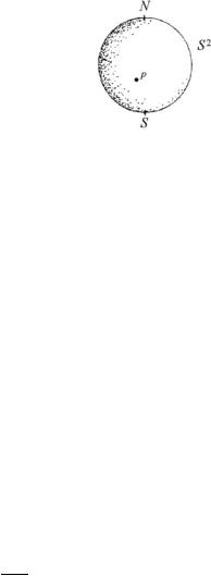
Fig. 2.19 The 2-sphere
and hence:
∞ |
d |
∞ |
d |
∞ |
t = − ck zS2−k |
|
= dk zSk |
|
= − dk zN2−k |
dzS |
dzS |
|||
k=0 |
|
k=0 |
|
k=0 |
The only way for (2.5.16) to be self consistent is to have:
k > 2 ck = dk = 0; c0 = −d2, c1 = −d1,
d |
∞ |
d |
|
|
= ck zNk |
|
|
dzN |
dzN |
||
|
k=0 |
(2.5.16) |
|
|
|
||
c2 |
= −d0 |
(2.5.17) |
|
This shows that the space of holomorphic sections of the tangent bundle T S2 is a finite dimensional vector space of dimension three spanned by the three differential operators:
L0 |
= −z |
d |
|
||||
|
|
|
|
|
|||
dz |
|
||||||
L1 |
= − |
d |
(2.5.18) |
||||
|
|
|
|||||
dz |
|||||||
L−1 |
= −z2 |
|
d |
|
|||
|
|
||||||
dz |
|
||||||
We will have more to say about these operators in the sequel.
What we have so far discussed can be summarized by stating the transformation rule of vector field components when we change coordinate patch form xμ to xμ :
∂xμ |
|
tμ x = tν (x) ∂xν |
(2.5.19) |
Indeed a convenient way of defining a fibre-bundle is provided by specifying the way its sections transform from one local trivialization to another one which amounts to giving all the transition functions. This method can be used to discuss the construction of the cotangent bundle.
2.5.2 The Lie Algebra of Vector Fields
In Sect. 2.3 we saw that the tangent space TpM at point p M of a manifold can be identified with the vector space of derivations of the algebra of germs (see
2.5 Tangent and Cotangent Bundles |
63 |
Definition 2.3.5). After gluing together all tangent spaces into the tangent bundle T M such an identification of tangent vectors with the derivations of an algebra can be extended from the local to the global level. The crucial observation is that the set of smooth functions on a manifold C∞(M ) constitutes an algebra with respect to point-wise multiplication just as the set of germs at point p. The vector fields, namely the sections of the tangent bundle, are derivations of this algebra. Indeed each vector field X Γ (T M , M ) is a linear map of the algebra C∞(M ) into itself:
X : C∞(M ) → C∞(M ) |
(2.5.20) |
that satisfies the analogue properties of those mentioned in (2.3.21) for tangent vectors, namely:
X(αf + βg) = αX(f ) + βX(g) |
|
X(f · g) = X(f ) · g + f · X(g) |
(2.5.21) |
α, β R (or C); f, g C∞(M ) |
|
On the other hand the set of vector fields, renamed for this reason: |
|
Diff(M ) ≡ Γ (T M , M ) |
(2.5.22) |
forms a Lie algebra with respect to the following Lie bracket operation: |
|
[X, Y]f = X Y(f ) − Y X(f ) |
(2.5.23) |
Indeed the set of vector fields is a vector space with respect the scalar numbers (R or C, depending on the type of manifold, real or complex), namely we can take linear combinations of the following form:
λ, μ R or C X, Y Diff(M ) : λX + μY Diff(M ) |
(2.5.24) |
having defined:
[λX + μY](f ) = λ X(f ) + μ Y(f ) , f C∞(M ) |
(2.5.25) |
Furthermore the operation (2.5.23) is the commutator of two maps and as such it is antisymmetric and satisfies the Jacobi identity.
The Lie algebra of vector fields is named Diff(M ) since each of its elements can be interpreted as the generator of an infinitesimal diffeomorphism of the manifold onto itself. As we are going to see Diff(M ) is a Lie algebra of infinite dimension, but it can contain finite dimensional subalgebras generated by particular vector fields. The typical example will be the case of the Lie algebra of a Lie group: this is the finite dimensional subalgebra G Diff(G) spanned by those vector fields defined on the Lie group manifold that have an additional property of invariance with respect to either left or right translations (see Chap. 3).

64 |
2 Manifolds and Fibre Bundles |
2.5.3 The Cotangent Bundle and Differential Forms
Let us recall that a differential 1-form in the point p M of a manifold M , namely an element ωp Tp M of the cotangent space over such a point was defined as a real valued linear functional over the tangent space at p, namely
ωp Hom(Tp M , R) |
(2.5.26) |
which implies: |
|
tp Tp M ωp : tp → ωp(tp ) R |
(2.5.27) |
The expression of ωp in a coordinate patch around p is: |
|
ωp = ωμ(p) dxμ |
(2.5.28) |
where dxμ(p) are the differentials of the coordinates and ωμ(p) are real numbers. We can glue together all the cotangent spaces and construct the cotangent bundles by stating that a generic smooth section of such a bundle is of the form (2.5.28) where ωμ(p) are now smooth functions of the base manifold point p. Clearly if we change coordinate system, an argument completely similar to that employed in the case of the tangent bundle tells us that the coefficients ωμ(x) transform as follows:
∂xν |
|
ωμ x = ων (x) ∂xμ |
(2.5.29) |
and (2.5.29) can be taken as a definition of the cotangent bundle T M , whose sections transform with the Jacobian matrix rather than with the inverse Jacobian matrix as the sections of the tangent bundle do (see (2.5.19)). So we can write the
Definition 2.5.3 A differential 1-form ω on a manifold M is a section of the cotangent bundle, namely ω Γ (T M , M ).
This means that a differential 1-form is a map: |
|
ω : Γ (T M , M ) → C∞(M ) |
(2.5.30) |
from the space of vector fields (i.e. the sections of the tangent bundle) to smooth functions. Locally we can write:
|
|
Γ (T M , M ) ω = ωμ(x) dxμ |
(2.5.31) |
|||||
|
|
Γ T M , M t = tμ(x) |
∂ |
|
||||
|
|
|
|
|
||||
|
|
∂xμ |
|
|||||
and we obtain |
|
|
|
|
|
|
|
|
|
= |
|
∂xν |
= |
|
|
|
|
ω(t) |
|
ωμ(x)tν (x) dxμ |
∂ |
|
|
ωμ(x)tμ(x) |
(2.5.32) |
|
|
|
|
||||||
using

2.5 Tangent and Cotangent Bundles |
65 |
dxμ |
∂ |
= δνμ |
(2.5.33) |
∂xν |
which is the statement that coordinate differentials and partial derivatives are dual bases for 1-forms and tangent vectors respectively.
Since T M is a vector bundle it is meaningful to consider the addition of its sections, namely the addition of vector fields and also their pointwise multiplication by smooth functions. Taking this into account we see that the map (2.5.30) used to define sections of the cotangent bundle, namely 1-forms is actually an F-linear map. This means the following. Considering any F-linear combination of two vector fields, namely:
f1t1 + f2t2, f1, f2 C∞(M ) t1, t2 Γ (T M , M ) |
(2.5.34) |
for any 1-form ω Γ (T M , M ) we have: |
|
ω(f1t1 + f2t2) = f1(p)ω(t1)(p) + f2(p)ω(t2)(p) |
(2.5.35) |
where p M is any point of the manifold M .
It is now clear that the definition of differential 1-form generalizes the concept of total differential of the germ of a smooth function. Indeed in an open neighborhood
U M of a point p we have: |
|
|
= |
|
|
||
|
|
|
p |
|
∂μf dxμ |
(2.5.36) |
|
|
f |
|
C∞(M ) |
df |
|
||
and the value of df at p on any tangent vector tp Tp M is defined to be: |
|
||||||
|
|
dfp (tp ) ≡ tp(f ) = tμ∂μf |
(2.5.37) |
||||
which is the directional derivative of the local function f along tp in the point p. If rather than the germ of a function we take a global function f C∞(M ) we realize that the concept of 1-form generalizes the concept of total differential of such a function. Indeed the total differential df fits into the definition of a 1-form, since for any vector field t Γ (T M , M ) we have:
df (t) = tμ(x)∂μf (x) ≡ tf C∞(M ) |
(2.5.38) |
A first obvious question is the following. Is any 1-form ω = ωμ(x) dxμ the differential of some function? The answer is clearly no and in any coordinate patch there
is a simple test to see whether this is the case or not. Indeed, if ωμ(1)
germ f |
|
p |
|
|
|
|
|
C∞(M ) then we must have: |
|
|
|||
|
|
1 |
∂μων(1) − ∂ν ωμ(1) = |
1 |
[∂μ, ∂ν ]f = 0 |
|
|
|
|
|
|
||
|
|
2 |
2 |
|||
= ∂μf for some
(2.5.39)
The left hand side of (2.5.39) are the components of what we will name a differential 2-form
ω(2) = ωμν(2) dxμ dxν |
(2.5.40) |