MICROSCOPY, CONFOCAL

NATHAN S. CLAXTON

THOMAS J. FELLERS

MICHAEL W. DAVIDSON

The Florida State University

Tallahassee, Florida

INTRODUCTION

The technique of laser scanning and spinning disk confocal fluorescence microscopy has become an essential tool in biology and the biomedical sciences, as well as in materials science due to attributes that are not readily available using other contrast modes with traditional optical microscopy (1–12). The application of a wide array of new synthetic and naturally occurring fluorochromes has made it possible to identify cells and submicroscopic cellular components with a high degree of specificity amid nonfluorescing material (13). In fact, the confocal microscope is often capable of revealing the presence of a single molecule (14). Through the use of multiply labeled specimens, different probes can simultaneously identify several target molecules simultaneously, both in fixed specimens and living cells and tissues (15). Although both conventional and confocal microscopes cannot provide spatial resolution below the diffraction limit of specific specimen features, the detection of fluorescing molecules below such limits is readily achieved.

The basic concept of confocal microscopy was originally developed by Minsky in the mid-1950s (patented in 1961) when he was a postdoctoral student at Harvard University (16,17). Minsky wanted to image neural networks in unstained preparations of brain tissue and was driven by the desire to image biological events as they occur in living systems. Minsky’s invention remained largely unnoticed, due most probably to the lack of intense light sources necessary for imaging and the computer horsepower required to handle large amounts of data. Following Minsky’s work, Egger and Petran (18) fabricated a multiplebeam confocal microscope in the late-1960s that utilized a spinning (Nipkow) disk for examining unstained brain sections and ganglion cells. Continuing in this arena, Egger went on to develop the first mechanically scanned confocal laser microscope, and published the first recognizable images of cells in 1973 (19). During the late-1970s and the 1980s, advances in computer and laser technology, coupled to new algorithms for digital manipulation of images, led to a growing interest in confocal microscopy (20).

Fortuitously, shortly after Minsky’s patent had expired, practical laser-scanning confocal microscope designs were translated into working instruments by several investigators. Dutch physicist Brakenhoff developed a scanning confocal microscope in 1979 (21), while almost simultaneously, Sheppard contributed to the technique with a theory of image formation (22). Wilson, Amos, and White nurtured the concept and later (during the late-1980s) demonstrated the utility of confocal imaging in the examination of fluorescent biological specimens (20,23). The first commercial instruments appeared in 1987. During the 1990s, advances in optics and electronics afforded more stable and powerful lasers, high efficiency scanning mirror

units, high throughput fiber optics, better thin-film dielectric coatings, and detectors having reduced noise characteristics (1). In addition, fluorochromes that were more carefully matched to laser excitation lines were beginning to be synthesized (13). Coupled to the rapidly advancing computer processing speeds, enhanced displays, and largevolume storage technology emerging in the late-1990s, the stage was set for a virtual explosion in the number of applications that could be targeted with laser scanning confocal microscopy.

Modern confocal microscopes can be considered as completely integrated electronic systems where the optical microscope plays a central role in a configuration that consists of one or more electronic detectors, a computer (for image display, processing, output, and storage), and several laser systems combined with wavelength selection devices and a beam scanning assembly. In most cases, integration between the various components is so thorough that the entire confocal microscope is often collectively referred to as a digital or video imaging system capable of producing electronic images (24). These microscopes are now being employed for routine investigations on molecules, cells, and living tissues that were not possible just a few years ago (15).

Confocal microscopy offers several advantages over conventional widefield optical microscopy, including the ability to control depth of field, elimination, or reduction of background information away from the focal plane (that leads to image degradation), and the capability to collect serial optical sections from thick specimens. The basic key to the confocal approach is the use of spatial filtering techniques to eliminate out-of-focus light or glare in specimens whose thickness exceeds the immediate plane of focus. There has been a tremendous explosion in the popularity of confocal microscopy in recent years (1–4,6,7), due in part to the relative ease with which extremely high quality images can be obtained from specimens prepared for conventional fluorescence microscopy, and the growing number of applications in cell biology that rely on imaging, both fixed and living cells and tissues. In fact, confocal technology is proving to be one of the most important advances ever achieved in optical microscopy.

In a conventional widefield optical epi-fluorescence microscope, secondary fluorescence emitted by the specimen often occurs through the excited volume and obscures resolution of features that lie in the objective focal plane (25). The problem is compounded by thicker specimens (>2 mm), which usually exhibit such a high degree of fluorescence emission that most of the fine detail is lost. Confocal microscopy provides only a marginal improvement in both axial (z; parallel to the microscope optical axis) and lateral (x and y; dimensions in the specimen plane) optical resolution, but is able to exclude secondary fluorescence in areas removed from the focal plane from resulting images (26– 28). Even though resolution is somewhat enhanced with confocal microscopy over conventional widefield techniques (1), it is still considerably less than that of the transmission electron microscope (TEM). In this regard, confocal microscopy can be considered a bridge between these two classical methodologies.

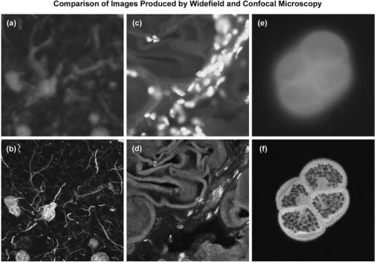
Illustrated in Fig. 1 are a series of images that compare selected viewfields in traditional widefield and laser

scanning confocal fluorescence microscopy. A thick (16 mm) section of fluorescently stained mouse hippocampus in widefield fluorescence exhibits a large amount of glare from fluorescent structures located above and below the focal plane (Fig. 1a). When imaged with a laser scanning confocal microscope (Fig. 1b), the brain thick section reveals a significant degree of structural detail. Likewise, widefield fluorescence imaging of rat smooth muscle fibers stained with a combination of Alexa Fluor dyes produce blurred images (Fig. 1c) lacking in detail, while the same specimen field (Fig. 1d) reveals a highly striated topography when viewed as an optical section with confocal microscopy. Autofluorescence in a sunflower (Helianthus annuus) pollen grain tetrad produces a similar indistinct outline of the basic external morphology (Fig. 1e), but yields no indication of the internal structure in widefield mode. In contrast, a thin optical section of the same grain (Fig. 1f) acquired with confocal techniques displays a dramatic difference between the particle core and the surrounding envelope. Collectively, the image comparisons in Fig. 1 dramatically depict the advantages of achieving very thin optical sections in confocal microscopy. The ability of this technique to eliminate fluorescence emission from regions removed from the focal plane offsets it from traditional forms of fluorescence microscopy.

PRINCIPLES OF CONFOCAL MICROSCOPY

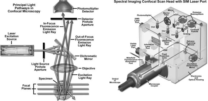
The confocal principle in epi-fluorescence laser scanning microscope is diagrammatically presented in Fig. 2. Coherent light emitted by the laser system (excitation source) passes through a pinhole aperture that is situated in a conjugate plane (confocal) with a scanning point on the specimen and a second pinhole aperture positioned in front of the detector (a photomultiplier tube). As the laser is reflected by a dichromatic mirror, and scanned across the specimen in a defined focal plane, secondary fluorescence emitted from points on the specimen (in the same focal plane) pass back through the dichromatic mirror, and are focused as a confocal point at the detector pinhole aperture.

The significant amount of fluorescence emission that occurs at points above and below the objective focal plane is not confocal with the pinhole (termed out-of-focus light rays in Fig. 2) and forms extended Airy disks in the aperture plane (29). Because only a small fraction of the out-of-focus fluorescence emission is delivered through the pinhole aperture, most of this extraneous light is not detected by the photomultiplier and does not contribute to the resulting image. The dichromatic mirror, barrier filter, and excitation filter perform similar functions to identical components in a widefield epi-fluorescence microscope (30).

Figure 2. Schematic diagram of the optical pathway and principal components in a laser scanning confocal microscope.

Refocusing the objective in a confocal microscope shifts the excitation and emission points on a specimen to a new plane that becomes confocal with the pinhole apertures of the light source and detector.

In traditional widefield epi-fluorescence microscopy, the entire specimen is subjected to intense illumination from an incoherent mercury or xenon arc-discharge lamp, and the resulting image of secondary fluorescence emission can be viewed directly in the eyepieces or projected onto the surface of an electronic array detector or traditional film plane. In contrast to this simple concept, the mechanism of image formation in a confocal microscope is fundamentally different (31). As discussed above, the confocal fluorescence microscope consists of multiple laser excitation sources, a scan head with optical and electronic components, electronic detectors (usually photomultipliers), and a computer for acquisition, processing, analysis, and display of images.

The scan head is at the heart of the confocal system and is responsible for rasterizing the excitation scans, as well as collecting the photon signals from the specimen that are required to assemble the final image (1,5–7). A typical scan head contains inputs from the external laser sources, fluorescence filter sets and dichromatic mirrors, a galvan- ometer-based raster scanning mirror system, variable pinhole apertures for generating the confocal image, and photomultiplier tube detectors tuned for different fluorescence wavelengths. Many modern instruments include diffraction gratings or prisms coupled with slits positioned near the photomultipliers to enable spectral imaging (also referred to as emission fingerprinting) followed by linear unmixing of emission profiles in specimens labeled with combinations of fluorescent proteins or fluorophores having overlapping spectra (32–38). The general arrangement of scan head components is presented in Fig. 3 for a typical commercial unit.

Figure 3. Three-channel spectral imaging laser scanning microscope confocal scan head with SIM scanner laser port. The SIM laser enables simultaneous excitation and imaging of the specimen for photobleaching or photoactivation experiments. Also illustrated are ports for a visible, ultraviolet (UV), and infrared (IR) laser, as well as an arc discharge lamp port for widefield observation.

In epi-illumination scanning confocal microscopy, the laser light source and photomultiplier detectors are both separated from the specimen by the objective, which functions as a well-corrected condenser and objective combination. Internal fluorescence filter components (e.g., the excitation and barrier filters and the dichromatic mirrors) and neutral density filters are contained within the scanning unit (see Fig. 3). Interference and neutral density filters are housed in rotating turrets or sliders that can be inserted into the light path by the operator. The excitation laser beam is connected to the scan unit with a fiber optic coupler followed by a beam expander that enables the thin laser beam wrist to completely fill the objective rear aperture (a critical requirement in confocal microscopy). Expanded laser light that passes through the microscope objective forms an intense diffraction-limited spot that is scanned by the coupled galvanometer mirrors in a raster pattern across the specimen plane (point scanning).

One of the most important components of the scanning unit is the pinhole aperture, which acts as a spatial filter at the conjugate image plane positioned directly in front of the photomultiplier (39). Several apertures of varying diameter are usually contained on a rotating turret that enables the operator to adjust pinhole size (and optical section thickness). Secondary fluorescence collected by the objective is descanned by the same galvanometer mirrors that form the raster pattern, and then passes through a barrier filter before reaching the pinhole aperture (40). The aperture serves to exclude fluorescence signals from out-of-focus features positioned above and below the focal plane, which are instead projected onto the aperture as Airy disks having a diameter much larger than those forming the image. These oversized disks are spread over

452 MICROSCOPY, CONFOCAL

Figure 4. Widefield versus confocal microscopy illumination volumes, demonstrating the difference in size between point scanning and widefield excitation light beams.

a comparatively large area so that only a small fraction of light originating in planes away from the focal point passes through the aperture. The pinhole aperture also serves to eliminate much of the stray light passing through the optical system. Coupling of aperture-limited point scanning to a pinhole spatial filter at the conjugate image plane is an essential feature of the confocal microscope.

When contrasting the similarities and differences between widefield and confocal microscopes, it is often useful to compare the character and geometry of specimen illumination utilized for each of the techniques. Traditional widefield epi-fluorescence microscope objectives focus a wide cone of illumination over a large volume of the specimen (41), which is uniformly and simultaneously illuminated (as illustrated in Fig. 4a). A majority of the fluorescence emission directed back toward the microscope is gathered by the objective (depending on the numerical aperture) and projected into the eyepieces or detector. The result is a significant amount of signal due to emitted background light and autofluorescence originating from areas above and below the focal plane, which seriously reduces resolution and image contrast.

The laser illumination source in confocal microscopy is first expanded to fill the objective rear aperture, and then focused by the lens system to a very small spot at the focal plane (Fig. 4b). The size of the illumination point ranges from 0.25 to 0.8 mm in diameter (depending on the objective numerical aperture) and 0.5 to 1.5 mm deep at the brightest intensity. Confocal spot size is determined by the microscope design, wavelength of incident laser light, objective characteristics, scanning unit settings, and the specimen (41). Figure 4 presents a comparison between the typical illumination cones of a widefield (Fig. 4a) and point scanning confocal (Fig. 4b) microscope at the same numerical aperture. The entire depth of the specimen over a wide area is illuminated by the widefield microscope, while the sample is scanned with a finely focused spot of illumination that is centered in the focal plane in the confocal microscope.

In laser scanning confocal microscopy, the image of an extended specimen is generated by scanning the focused beam across a defined area in a raster pattern controlled by two high speed oscillating mirrors driven with galvanometer motors. One of the mirrors moves the beam from left to right along the x lateral axis, while the other translates the beam in the y direction. After each single scan along the x axis, the beam is rapidly transported back to the starting point and shifted along the y axis to begin a new scan in a process termed flyback (42). During the flyback operation, image information is not collected. In

this manner, the area of interest on the specimen in a single focal plane is excited by laser illumination from the scanning unit.

As each scan line passes along the specimen in the lateral focal plane, fluorescence emission is collected by the objective and passed back through the confocal optical system. The speed of the scanning mirrors is very slow relative to the speed of light, so the secondary emission follows a light path along the optical axis that is identical to the original excitation beam. Return of fluorescence emission through the galvanometer mirror system is referred to as descanning (40,42). After leaving the scanning mirrors, the fluorescence emission passes directly through the dichromatic mirror and is focused at the detector pinhole aperture. Unlike the raster scanning pattern of excitation light passing over the specimen, fluorescence emission remains in a steady position at the pinhole aperture, but fluctuates with respect to intensity over time as the illumination spot traverses the specimen producing variations in excitation.

Fluorescence emission that is passed through the pinhole aperture is converted into an analog electrical signal having a continuously varying voltage (corresponding to intensity) by the photomultiplier. The analog signal is periodically sampled and converted into pixels by an analog-to-digital (A/D) converter housed in the scanning unit or the accompanying electronics cabinet. The image information is temporarily stored in an image frame buffer card in the computer and displayed on the monitor. Note that the confocal image of a specimen is reconstructed, point by point, from emission photon signals by the photomultiplier and accompanying electronics, yet never exists as a real image that can be observed through the microscope eyepieces.

LASER SCANNING CONFOCAL MICROSCOPE CONFIGURATION

Basic microscope optical system characteristics have remained fundamentally unchanged for many decades due to engineering restrictions on objective design, the static properties of most specimens, and the fact that resolution is governed by the wavelength of light (1–10). However, fluorescent probes that are employed to add contrast to biological specimens and, and other technologies associated with optical microscopy techniques, have improved significantly. The explosive growth and development of the confocal approach is a direct result of a renaissance in optical microscopy that has been largely fueled by advances in modern optical and electronics technology. Among these are stable multiwavelength laser systems that provide better coverage of the uv, visible, and nearIR spectral regions, improved interference filters (including dichromatic mirrors, barrier, and excitation filters), sensitive low noise wide-band detectors, and far more powerful computers. The latter are now available with relatively low cost memory arrays, image analysis software packages, high resolution video displays, and high quality digital image printers. The flow of information through a modern confocal microscope is presented diagrammatically in Fig. 5 (2).

Figure 5. Confocal microscope configuration and information flow schematic diagram.

Although many of these technologies have been developed independently for a variety of specifically targeted applications, they have been incorporated gradually into mainstream commercial confocal microscopy systems. In current microscope systems, classification of designs is based on the technology utilized to scan specimens (7). Scanning can be accomplished either by translating the stage in the x, y, and z directions while the laser illumination spot is held in a fixed position, or the beam itself can be raster-scanned across the specimen. Because threedimensional (3D) translation of the stage is cumbersome and prone to vibration, most modern instruments employ some type of beam-scanning mechanism.

In modern confocal microscopes, two fundamentally different techniques for beam scanning have been developed. Single-beam scanning, one of the more popular methods employed in a majority of the commercial laser scanning microscopes (43), uses a pair of computer-con- trolled galvanometer mirrors to scan the specimen in a raster pattern at a rate of approximately one frame per second. Faster scanning rates (to near video speed) can be achieved using acoustooptic devices or oscillating mirrors. In contrast, multiple-beam scanning confocal microscopes are equipped with a spinning Nipkow disk containing an array of pinholes and microlenses (44–46). These instruments often use arc-discharge lamps for illumination instead of lasers to reduce specimen damage and enhance the detection of low fluorescence levels during real-time image collection. Another important feature of the multiplebeam microscopes is their ability to readily capture images with an array detector, such as a charge-coupled device (CCD) camera system (47).

All modern laser scanning confocal microscope designs are centered on a conventional upright or inverted research level optical microscope. However, instead of the standard tungsten–halogen or mercury (xenon) arcdischarge lamp, one or more laser systems are used as a light source to excite fluorophores in the specimen. Image information is gathered point by point with a specialized detector, such as a photomultiplier tube or avalanche photodiode, and then digitized for processing by the host

computer, which also controls the scanning mirrors and/or other devices to facilitate the collection and display of images. After a series of images (usually serial optical sections) has been acquired and stored on digital media, analysis can be conducted utilizing numerous image processing software packages available on the host or a secondary computer.

ADVANTAGES AND DISADVANTAGES OF CONFOCAL MICROSCOPY

The primary advantage of laser scanning confocal microscopy is the ability to serially produce thin (0.5–1.5 mm) optical sections through fluorescent specimens that have a thickness ranging up to 50 mm or more (48). The image series is collected by coordinating incremental changes in the microscope fine focus mechanism (using a stepper motor) with sequential image acquisition at each step. Image information is restricted to a well-defined plane, rather than being complicated by signals arising from remote locations in the specimen. Contrast and definition are dramatically improved over widefield techniques due to the reduction in background fluorescence and improved signal to noise (48). Furthermore, optical sectioning eliminates artifacts that occur during physical sectioning and fluorescent staining of tissue specimens for traditional forms of microscopy. The noninvasive confocal optical sectioning technique enables the examination of both living and fixed specimens under a variety of conditions with enhanced clarity.

With most confocal microscopy software packages, optical sections are not restricted to the perpendicular lateral (x–y) plane, but can also be collected and displayed in transverse planes (1,5–8,49). Vertical sections in the x–z and y–z planes (parallel to the microscope optical axis) can be readily generated by most confocal software programs. Thus, the specimen appears as if it had been sectioned in a plane that is perpendicular to the lateral axis. In practice, vertical sections are obtained by combining a series of x–y scans taken along the z axis with the software, and then projecting a view of fluorescence intensity as it would appear should the microscope hardware have been capable of physically performing a vertical section.

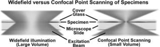
A typical stack of optical sections (often termed a z series) through a Lodgepole Pine tree pollen grain revealing internal variations in autofluorescence emission wavelengths is illustrated in Fig. 6. Optical sections were gathered in 1.0 mm steps perpendicular to the z axis (microscope optical axis) using a laser combiner featuring an argon ion (488 nm; green fluorescence), a green helium– neon (543 nm; red fluorescence), and a red helium–neon (633 nm; fluorescence pseudocolored blue) laser system. Pollen grains from this and many other species range between 10 and 40 mm in diameter and often yield blurred images in wide-field fluorescence microscopy (see Fig. 1c), which lack information about internal structural details. Although only 12 of the >36 images collected through this series are presented in the figure, they represent individual focal planes separated by a distance of 3 mm and provide a good indication of the internal grain structure.

454 MICROSCOPY, CONFOCAL

Figure 6. Lodgepole pine (Pinus contorta) pollen grain optical sections. Bulk pollen was mounted in CytoSeal 60 and imaged with a 100 oil immersion objective (no zoom) in 1 mm axial steps. Each image in the sequence (1–12) represents the view obtained from steps of 3 mm.

In specimens more complex than a pollen grain, complex interconnected structural elements can be difficult to discern from a large series of optical sections sequentially acquired through the volume of a specimen with a laser scanning confocal microscope. However, once an adequate series of optical sections has been gathered, it can be further processed into a 3D representation of the specimen using volume-rendering computational techniques (50–53). This approach is now in common use to help elucidate the numerous interrelationships between structure and function of cells and tissues in biological investigations (54). In order to ensure that adequate data is collected to produce a representative volume image, the optical sections should be recorded at the appropriate axial (z step) intervals so that the actual depth of the specimen is reflected in the image.

Most of the software packages accompanying commercial confocal instruments are capable of generating composite and multidimensional views of optical section data acquired from z-series image stacks. The 3D software packages can be employed to create either a single 3D representation of the specimen (Fig. 7) or a video (movie) sequence compiled from different views of the specimen volume. These sequences often mimic the effect of rotation or similar spatial transformation that enhances the appreciation of the specimen’s 3D character. In addition, many software packages enable investigators to conduct measurements of length, volume, and depth, and specific parameters of the images, such as opacity, can be interactively altered to reveal internal structures of interest at differing levels within the specimen (54).

Typical 3D representations of several specimens examined by serial optical sectioning are presented in Fig. 7. A series of sunflower pollen grain optical sections was combined to produce a realistic view of the exterior surface (Fig. 7a) as it might appear if being examined by a scanning electron microscope (SEM). The algorithm utilized to construct the 3D model enables the user to rotate the

Figure 7. Three-dimensional volume renders from confocal microscopy optical sections. (a) Autofluorescence in a series of sunflower pollen grain optical sections was combined to produce a realistic view of the exterior surface. (b) Mouse lung tissue thick (16 mm)section. (c)Ratbrain thick section. These specimens were each labeled with several fluorophores (blue, green, and red fluorescence) and the volume renders were created from a stack of 30–45 optical sections. (d) Autofluorescence in a thin section of fern root.

pollen grain through 3608 for examination. Similarly, thick sections (16 mm) of lung tissue and rat brain are presented in Fig. 7b and 7c, respectively. These specimens were each labeled with several fluorophores (blue, green, and red fluorescence) and created from a stack of 30–45 optical sections. Autofluorescence in plant tissue was utilized to produce the model illustrated in Fig. 7d of a fern root section.

In many cases, a composite or projection view produced from a series of optical sections provides important information about a 3D specimen than a multidimensional view (54). For example, a fluorescently labeled neuron having numerous thin, extended processes in a tissue section is difficult (if not impossible) to image using wide-field techniques due to out-of-focus blur. Confocal thin sections of the same neuron each reveal portions of several extensions, but these usually appear as fragmented streaks and dots and lack continuity (53). Composite views created by flattening a series of optical sections from the neuron will reveal all of the extended processes in sharp focus with well-defined continuity. Structural and functional analysis of other cell and tissue sections also benefits from composite views as opposed to, or coupled with, 3D volume rendering techniques.

Advances in confocal microscopy have made possible multidimensional views (54) of living cells and tissues that include image information in the x, y, and z dimensions as a function of time and presented in multiple colors (using two or more fluorophores). After volume processing of individual image stacks, the resulting data can be displayed as 3D multicolor video sequences in real time. Note that unlike conventional widefield microscopy, all fluorochromes in multiply labeled specimens appear in register

using the confocal microscope. Temporal data can be collected either from time-lapse experiments conducted over extended periods or through real-time image acquisition in smaller frames for short periods of time. The potential for using multidimensional confocal microscopy as a powerful tool in cellular biology is continuing to grow as new laser systems are developed to limit cell damage and computer processing speeds and storage capacity improves.

Additional advantages of scanning confocal microscopy include the ability to adjust magnification electronically by varying the area scanned by the laser without having to change objectives. This feature is termed the zoom factor, and is usually employed to adjust the image spatial resolution by altering the scanning laser sampling period (1,2,8,40,55). Increasing the zoom factor reduces the specimen area scanned and simultaneously reduces the scanning rate. The result is an increased number of samples along a comparable length (55), which increases both the image spatial resolution and display magnification on the host computer monitor. Confocal zoom is typically employed to match digital image resolution (8,40,55) with the optical resolution of the microscope when low numerical aperture and magnification objectives are being used to collect data.

Digitization of the sequential analog image data collected by the confocal microscope photomultiplier (or similar detector) facilitates computer image processing algorithms by transforming the continuous voltage stream into discrete digital increments that correspond to variations in light intensity. In addition to the benefits and speed that accrue from processing digital data, images can be readily prepared for print output or publication. In carefully controlled experiments, quantitative measurements of spatial fluorescence intensity (either statically or as a function of time) can also be obtained from the digital data.

Disadvantages of confocal microscopy are limited primarily to the limited number of excitation wavelengths available with common lasers (referred to as laser lines), which occur over very narrow bands and are expensive to produce in the UV region (56). In contrast, conventional widefield microscopes use mercuryor xenon-based arcdischarge lamps to provide a full range of excitation wavelengths in the UV, visible, and near-IR spectral regions. Another downside is the harmful nature (57) of high intensity laser irradiation to living cells and tissues, an issue that has recently been addressed by multiphoton and Nipkow disk confocal imaging. Finally, the high cost of purchasing and operating multiuser confocal microscope systems (58), which can range up to an order of magnitude higher than comparable widefield microscopes, often limits their implementation in smaller laboratories. This problem can be easily overcome by cost-shared microscope systems that service one or more departments in a core facility. The recent introduction of personal confocal systems has competitively driven down the price of low end confocal microscopes and increased the number of individual users.

CONFOCAL MICROSCOPE LIGHT DETECTORS

In modern widefield fluorescence and laser scanning confocal optical microscopy, the collection and measurement of

secondary emission gathered by the objective can be accomplished by several classes of photosensitive detectors (59), including photomultipliers, photodiodes, and solid-state CCDs. In confocal microscopy, fluorescence emission is directed through a pinhole aperture positioned near the image plane to exclude light from fluorescent structures located away from the objective focal plane, thus reducing the amount of light available for image formation, as discussed above. As a result, the exceedingly low light levels most often encountered in confocal microscopy necessitate the use of highly sensitive photon detectors that do not require spatial discrimination, but instead respond very quickly with a high level of sensitivity to a continuous flux of varying light intensity.

Photomultipliers, which contain a photosensitive surface that captures incident photons and produces a stream of photoelectrons to generate an amplified electric charge, are the popular detector choice in many commercial confocal microscopes (59–61). These detectors contain a critical element, termed a photocathode, capable of emitting electrons through the photoelectric effect (the energy of an absorbed photon is transferred to an electron) when exposed to a photon flux. The general anatomy of a photomultiplier consists of a classical vacuum tube in which a glass or quartz window encases the photocathode and a chain of electron multipliers, known as dynodes, followed by an anode to complete the electrical circuit (62). When the photomultiplier is operating, current flowing between the anode and ground (zero potential) is directly proportional to the photoelectron flux generated by the photocathode when it is exposed to incident photon radiation.

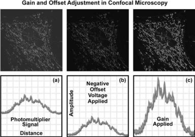
In a majority of commercial confocal microscopes, the photomultiplier is located within the scan head or an external housing, and the gain, offset, and dynode voltage are controlled by the computer software interface to the detector power supply and supporting electronics (7). The voltage setting is used to regulate the overall sensitivity of the photomultiplier, and can be adjusted independently of the gain and offset values. The latter two controls are utilized to adjust the image intensity values to ensure that the maximum number of gray levels is included in the output signal of the photomultiplier. Offset adds a positive or negative voltage to the output signal, and should be adjusted so that the lowest signals are near the photomultiplier detection threshold (40). The gain circuit multiplies the output voltage by a constant factor so that the maximum signal values can be stretched to a point just below saturation. In practice, offset should be applied first before adjusting the photomultiplier gain (8,40). After the signal has been processed by the analog-to-digital converter, it is stored in a frame buffer and ultimately displayed on the monitor in a series of gray levels ranging from black (no signal) to white (saturation). Photomultipliers with a dynamic range of 10 or 12 bits are capable of displaying 1024 or 4096 gray levels, respectively. Accompanying image files also have the same number of gray levels. However, the photomultipliers used in a majority of the commercial confocal microscopes have a dynamic range limited to 8 bits or 256 gray levels, which in most cases, is adequate for handling the typical number of photons scanned per pixel (63).

456 MICROSCOPY, CONFOCAL

Changes to the photomultiplier gain and offset levels should not be confused with postacquisition image processing to adjust the levels, brightness, or contrast in the final image. Digital image processing techniques can stretch existing pixel values to fill the black-to-white display range, but cannot create new gray levels (40). As a result, when a digital image captured with only 200 out of a possible 4096 gray levels is stretched to fill the histogram (from black to white), the resulting processed image appears grainy. In routine operation of the confocal microscope, the primary goal is to fill as many of the gray levels during image acquisition and not during the processing stages.

The offset control is used to adjust the background level to a position near 0 V (black) by adding a positive or negative voltage to the signal. This ensures that dark features in the image are very close to the black level of the host computer monitor. Offset changes the amplitude of the entire voltage signal, but since it is added to or subtracted from the total signal, it does not alter the voltage differential between the high and low voltage amplitudes in the original signal. For example, with a signal ranging from 4 to 18 V that is modified with an offset setting of 4 V, the resulting signal spans 0–14 V, but the difference remains 14 V.

Figure 8 presents a series of diagrammatic schematics of the unprocessed and adjusted output signal from a photomultiplier and the accompanying images captured with a confocal microscope of a living adherent culture of Indian Muntjac deer skin fibroblast cells treated with MitoTracker Red CMXRos, which localizes specifically in the mitochondria. Figure 8a illustrates the raw confocal image along with the signal from the photomultiplier. After applying a negative offset voltage to the photomultiplier, the signal and image appear in Fig. 8b. Note that as the signal is shifted to lower intensity values, the image becomes darker (upper frame in Fig. 8b). When the gain is adjusted to the full intensity range (Fig. 8c), the image exhibits a significant amount of detail with good contrast and high resolution.

The photomultiplier gain adjustment is utilized to electronically stretch the input signal by multiplying with a constant factor prior to digitization by the analog-to-digital converter (40). The result is a more complete representation of gray level values between black and white, and an increase in apparent dynamic range. If the gain setting is increased beyond the optimal point, the image becomes grainy, but this maneuver is sometimes necessary to capture the maximum number of gray levels present in the image. Advanced confocal microscopy software packages ease the burden of gain and offset adjustment by using a pseudocolor display function to associate pixel values with gray levels on the monitor. For example, the saturated pixels (255) can be displayed in yellow or red, while blackevel pixels (0) are shown in blue or green, with intermediate gray levels displayed in shades of gray representing their true values. When the photomultiplier output is properly adjusted, just a few red (or yellow) and blue (or green) pixels are present in the image, indicating that the full dynamic range of the photomultiplier is being utilized.

Established techniques in the field of enhanced night vision have been applied with dramatic success to photomultipliers designed for confocal microscopy (63,64). Several manufacturers have collaborated to fabricate a headon photomultiplier containing a specialized prism system that assists in the collection of photons. The prism operates by diverting the incoming photons to a pathway that promotes total internal reflection in the photomultiplier envelope adjacent to the photocathode. This configuration increases the number of potential interactions between the photons and the photocathode, resulting in an increase in quantum efficiency by more than a factor of 2 in the green spectral region, 4 in the red region, and even higher in the IR (59). Increasing the ratio of photoelectrons generated to the number of incoming photons serves to increase the electrical current from the photomultiplier, and to produce a higher sensitivity for the instrument.

Photomultipliers are the ideal photometric detectors for confocal microscopy due to their speed, sensitivity, high signal/noise ratio, and adequate dynamic range (59–61).

High end confocal microscope systems have several photomultipliers that enable simultaneous imaging of different fluorophores in multiply labeled specimens. Often, an additional photomultiplier is included for imaging the specimen with transmitted light using differential interference or phase-contrast techniques. In general, confocal microscopes contain three photomultipliers for the fluorescence color channels (red, green, and blue; each with a separate pinhole aperture) utilized to discriminate between fluorophores, along with a fourth for transmitted or reflected light imaging. Signals from each channel can be collected simultaneously and the images merged into a single profile that represents the real colors of the stained specimen. If the specimen is also imaged with a brightfield contrastenhancing technique, such as differential interference contrast (65), the fluorophore distribution in the fluorescence image can be overlaid onto the brightfield image to determine the spatial location of fluorescence emission within the structural domains.

ACOUSTOOPTIC TUNABLE FILTERS IN CONFOCAL MICROSCOPY

The integration of optoelectronic technology into confocal microscopy has provided a significant enhancement in the versatility of spectral control for a wide variety of fluorescence investigations. The acoustooptic tunable filter (AOTF) is an electrooptical device that functions as an electronically tunable excitation filter to simultaneously modulate the intensity and wavelength of multiple laser lines from one or more sources (66). Devices of this type rely on a specialized birefringent crystal whose optical properties vary upon interaction with an acoustic wave. Changes in the acoustic frequency alter the diffraction properties of the crystal, enabling very rapid wavelength tuning, limited only by the acoustic transit time across the crystal.

An acoustooptic tunable filter designed for microscopy typically consists of a tellurium dioxide or quartz anisotropic crystal to which a piezoelectric transducer is bonded (67–70). In response to the application of an oscillating radio frequency (RF) electrical signal, the transducer generates a high frequency vibrational (acoustic) wave that propagates into the crystal. The alternating ultrasonic acoustic wave induces a periodic redistribution of the refractive index through the crystal that acts as a transmission diffraction grating or Bragg diffracter to deviate a portion of incident laser light into a first-order beam, which is utilized in the microscope (or two first-order beams when the incident light is nonpolarized). Changing the frequency of the transducer signal applied to the crystal alters the period of the refractive index variation, and therefore, the wavelength of light that is diffracted. The relative intensity of the diffracted beam is determined by the amplitude (power) of the signal applied to the crystal.

In the traditional fluorescence microscope configuration, including many confocal systems, spectral filtering of both excitation and emission light is accomplished utilizing thin-film interference filters (7). These filters are limiting in several respects. Because each filter has a fixed central wavelength and passband, several filters must be

utilized to provide monochromatic illumination for multispectral imaging, as well as to attenuate the beam for intensity control, and the filters are often mechanically interchanged by a rotating turret mechanism. Interference filter turrets and wheels have the disadvantages of limited wavelength selection, vibration, relatively slow switching speed, and potential image shift (70). They are also susceptible to damage and deterioration caused by exposure to heat, humidity, and intense illumination, which changes their spectral characteristics over time. In addition, the utilization of filter wheels for illumination wavelength selection has become progressively more complex and expensive as the number of lasers being employed has increased with current applications.

Rotation of filter wheels and optical block turrets introduces mechanical vibrations into the imaging and illumination system, which consequently requires a time delay for damping of perhaps 50 ms, even if the filter transition itself can be accomplished more quickly. Typical filter change times are considerably slower in practice, however, and range on the order of 0.1–0.5 s. Mechanical imprecision in the rotating mechanism can introduce registration errors when sequentially acquired multicolor images are processed. Furthermore, the fixed spectral characteristics of interference filters do not allow optimization for different fluorophore combinations, nor for adaptation to new fluorescent dyes, limiting the versatility of both the excitation and detection functions of the microscope. Introduction of the AOTF to confocal systems overcomes most of the filter wheel disadvantages by enabling rapid simultaneous electronic tuning and intensity control of multiple laser lines from several lasers.

As applied in laser scanning confocal microscopy, one of the most significant benefits of the AOTF is its capability to replace much more complex and unwieldy filter mechanisms for controlling light transmission, and to apply intensity modulation for wavelength discrimination purposes (67,70). The ability to perform extremely rapid adjustments in the intensity and wavelength of the diffracted beam gives the AOTF unique control capabilities. By varying the illumination intensity at different wavelengths, the response of multiple fluorophores, for example, can be balanced for optimum detection and recording (71). In addition, digital signal processors along with phase and frequency lock-in techniques can be employed to discriminate emission from multiple fluorophores or to extract low level signals from background.

A practical light source configuration scheme utilizing an acoustooptic tunable filter for confocal microscopy is illustrated in Fig. 9. The output of three laser systems (violet diode, argon, and argon–krypton) are combined by dichromatic mirrors and directed through the AOTF, where the first-order diffracted beam (green) is collinear and is launched into a single-mode fiber. The undiffracted laser beams (violet, green, yellow, and red) exit the AOTF at varying angles and are absorbed by a beam stop (not illustrated). The major lines (wavelengths) produced by each laser are indicated (in nm) beneath the hot and cold mirrors. The dichromatic mirror reflects wavelengths < 525 nm and transmits longer wavelengths. Two longer wavelength lines produced by the argon–krypton laser

458 MICROSCOPY, CONFOCAL

Figure 9. Configuration scheme utilizing an AOTF for laser intensity control and wavelength selection in confocal microscopy.

(568 and 648 nm) are reflected by the hot mirror, while the output of the argon laser (458, 476, 488, and 514 nm) is reflected by the dichromatic mirror and combined with the transmitted light from the argon–krypton laser. Output from the violet diode laser (405 nm) is reflected by the cold mirror and combined with the longer wavelengths from the other two lasers, which are transmitted through the mirror.

Because of the rapid optical response from the AOTF crystal to the acoustic transducer, the acoustooptic interaction is subject to abrupt transitions resembling a rectangular rather than sinusoidal waveform (66). This results in the occurrence of sidelobes in the AOTF passband on either side of the central transmission peak. Under ideal acoustooptic conditions, these sidelobes should be symmetrical about the central peak, with the first lobe having 4.7% of the central peak’s intensity. In practice, the sidelobes are commonly asymmetrical and exhibit other deviations from predicted structure caused by variations in the acoustooptic interaction, among other factors. In order to reduce the sidelobes in the passband to insignificant levels, several types of amplitude apodization of the acoustic wave are employed (66,67), including various window functions, which have been found to suppress the highest sidelobe by 30–40 dB. One method that can be used in reduction of sidelobe level with noncollinear AOTFs is to apply spatial apodization by means of weighted excitation of the transducer. In the collinear AOTF, a different approach has been employed, which introduces an acoustic pulse, apodized in time, into the filter crystal.

The effective linear aperture of an AOTF is limited by the acoustic beam height in one dimension (ID) and by the acoustic attenuation across the optical aperture (the acoustic transit distance) in the other dimension (67). The height of the acoustic beam generated within the AOTF crystal is determined by the performance and physical properties of the acoustic transducer. Acoustic attenuation in crystalline materials, such as tellurium dioxide, is proportional to the square of acoustic frequency, and is therefore a more problematic limitation to linear aperture size in the shorter wavelength visible light range, which requires higher RF frequencies for tuning. Near-IR and IR radiation produces

less restrictive limitations because of the lower acoustic frequencies associated with diffraction of these longer wavelengths.

The maximum size of an individual acoustic transducer is constrained by performance and power requirements in addition to the geometric limitations of the instrument configuration, and AOTF designers may use an array of transducers bonded to the crystal in order to increase the effective lateral dimensions of the propagating acoustic beam, and to enlarge the area of acoustooptic interaction (66,67,70). The required drive power is one of the most important variables in acoustooptic design, and generally increases with optical aperture and for longer wavelengths. In contrast to acoustic attenuation, which is reduced in the IR spectral range, the higher power required to drive transducers for infrared AOTFs is one of the greatest limitations in these devices. High drive power levels result in heating of the crystal, which can cause thermal drift and instability in the filter performance (66). This is particularly a problem when acoustic power and frequency are being varied rapidly over a large range, and the crystal temperature does not have time to stabilize, producing transient variations in refractive index. If an application requires wavelength and intensity stability and repeatability, the AOTF should be maintained at a constant temperature. One approach taken by equipment manufacturers to minimize this problem is to heat the crystal above ambient temperature, to a level at which it is relatively unaffected by the additional thermal input of the transducer drive power. An alternative solution is to house the AOTF in a thermoelectrically cooled housing that provides precise temperature regulation. Continuing developmental efforts promise to lead to new materials that can provide relatively large apertures combined with effective separation of the filtered and unfiltered beams without use of polarizers, while requiring a fraction of the typical device drive power.

In a noncollinear AOTF, which spatially separates the incident and diffracted light paths, the deflection angle (the angle separating diffracted and undiffracted light beams exiting the crystal) is an additional factor limiting the effective aperture of the device (67). As discussed previously, the deflection angle is greater for crystals having greater birefringence, and determines in part the propagation distance required for adequate separation of the diffracted and undiffracted beams to occur after exiting the crystal. The required distance is increased for larger entrance apertures, and this imposes a practical limit on maximum aperture size because of constraints on the physical dimensions of components that can be incorporated into a microscope system. The angular aperture is related to the total light collecting power of the AOTF, an important factor in imaging systems, although in order to realize the full angular aperture without the use of polarizers in the noncollinear AOTF, its value must be smaller than the deflection angle. Because the acoustooptic tunable filter is not an image-forming component of the microscope system (it is typically employed for source filtering), there is no specific means of evaluating the spatial resolution for this type of device (70). However, the AOTF may restrict the attainable spatial resolution of the imaging system

because of its limited linear aperture size and acceptance angle, in the same manner as other optical components. Based on the Rayleigh criterion and the angular and linear apertures of the AOTF, the maximum number of resolvable image elements may be calculated for a given wavelength, utilizing different expressions for the polar and azimuthal planes. Although diffraction limited resolution can be attained in the azimuthal plane, dispersion in the AOTF limits the resolution in the polar plane, and measures must be taken to suppress this factor for optimum performance. The dependence of deflection angle on wavelength can produce one form of dispersion, which is typically negligible when tuning is performed within a relatively narrow bandwidth, but significant in applications involving operation over a broad spectral range. Changes in deflection angle with wavelength can result in image shifts during tuning, producing errors in techniques, such as ratio imaging of fluorophores excited at different wavelengths, and in other multispectral applications. When the image shift obeys a known relationship to wavelength, corrections can be applied through digital processing techniques (1,7). Other effects of dispersion, including reduced angular resolution, may result in image degradation, such as blurring, that requires more elaborate measures to suppress.

SUMMARY OF AOTF BENEFITS IN CONFOCAL MICROSCOPY

Considering the underlying principles of operation and performance factors that relate to the application of AOTFs in imaging systems, a number of virtues from such devices for light control in fluorescence confocal microscopy are apparent. Several benefits of the AOTF combine to greatly

enhance the versatility of the latest generation of confocal instruments, and these devices are becoming increasing popular for control of excitation wavelength ranges and intensity. The primary characteristic that facilitates nearly every advantage of the AOTF is its capability to allow the microscopist control of the intensity and/or illumination wavelength on a pixel-by-pixel basis while maintaining a high scan rate (7). This single feature translates into a wide variety of useful analytical microscopy tools, which are even further enhanced in flexibility when laser illumination is employed.

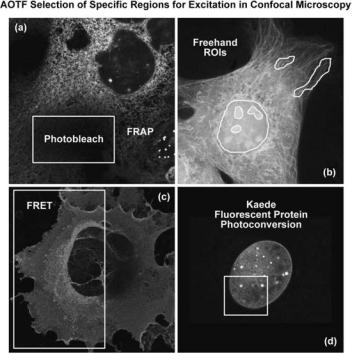
One of the most useful AOTF functions allows the selection of small user-defined specimen areas (commonly termed regions of interest; ROI) that can be illuminated with either greater or lesser intensity, and at different wavelengths, for precise control in photobleaching techniques, excitation ratio studies, resonance energy-transfer investigations, or spectroscopic measurements (see Fig. 10). The illumination intensity can not only be increased in selected regions for controlled photobleaching experiments (71–73), but can be attenuated in desired areas in order to minimize unnecessary photobleaching. When the illumination area is under AOTF control, the laser exposure is restricted to the scanned area by default, and the extremely rapid response of the device can be utilized to provide beam blanking during the flyback interval of the galvanometer scanning mirror cycle, further limiting unnecessary specimen exposure. In practice, the regions of excitation are typically defined by freehand drawing or using tools to produce defined geometrical shapes in an overlay plane on the computer monitor image. Some systems allow any number of specimen areas to be defined for laser exposure, and the laser intensity to be set to different levels for each area, in intensity increments as small as 0.1%. When the

460 MICROSCOPY, CONFOCAL

AOTF is combined with multiple lasers and software that allows time course control of sequential observations, timelapse experiments can be designed to acquire data from several different areas in a single experiment, which might, for example, be defined to correspond to different cellular organelles.

Figure 10 illustrates several examples of several userdefined ROIs that were created for advanced fluorescence applications in laser scanning confocal microscopy. In each image, the ROI is outlined with a yellow border. The rat kangaroo kidney epithelial cell (PtK2 line) presented in Fig. 10a has a rectangular area in the central portion of the cytoplasm that has been designated for photobleaching experiments. Fluorophores residing in this region can be selectively destroyed by high power laser intensity, and the subsequent recovery of fluorescence back into the photobleached region monitored for determination of diffusion coefficients. Several freehand ROIs are illustrated in Fig. 10b, which can be targets for selective variation of illumination intensities or photobleaching and photoactivation experiments. Fluorescence resonance energytransfer emission ratios can be readily determined using selected regions in confocal microscopy by observing the effect of bleaching the acceptor fluorescence in these areas (Fig. 10c; African green monkey kidney epithelial cells labeled with Cy3 and Cy5 conjugated to cholera toxin, which localizes in the plasma membrane). The AOTF control of laser excitation in selected regions with confocal microscopy is also useful for investigations of protein diffusion in photoactivation studies (74–76) using fluorescent proteins, as illustrated in Fig. 10d. This image frame presents the fluorescence emission peak of the Kaede protein as it shifts from green to red in HeLa (human

cervical carcinoma) cell nuclei using selected illumination (yellow box) with a 405 nanometer violet–blue diode laser.

The rapid intensity and wavelength switching capabilities of the AOTF enable sequential line scanning of multiple laser lines to be performed in which each excitation wavelength can be assigned a different intensity in order to balance the various signal levels for optimum imaging (77). Sequential scanning of individual lines minimizes the time differential between signal acquisitions from the various fluorophores while reducing crossover, which can be a significant problem with simultaneous multiple-wavelength excitation (Fig. 11). The synchronized incorporation of multiple fluorescent probes into living cells has grown into an extremely valuable technique for study of protein– protein interactions, and the dynamics of macromolecular complex assembly. The refinement of techniques for incorporating green fluorescent protein (GFP) and its numerous derivatives into the protein-synthesizing mechanisms of the cell has revolutionized living cell experimentation (78–80). A major challenge in multipleprobe studies using living tissue is the necessity to acquire the complete multispectral data set quickly enough to minimize specimen movement and molecular changes that might distort the true specimen geometry or dynamic sequence of events (32–34). The AOTF provides the speed and versatility to control the wavelength and intensity illuminating multiple specimen regions, and to simultaneously or sequentially scan each at sufficient speed to accurately monitor dynamic cellular processes.

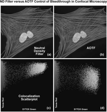
A comparison between the application of AOTFs and neutral density filters (78) to control spectral separation of fluorophore emission spectra in confocal microscopy is presented in Fig. 11. The specimen is a monolayer culture

of adherent human lung fibroblast (MRC-5 line) cells stained with Texas Red conjugated to phalloidin (targeting the filamentous actin network) and SYTOX Green (staining DNA in the nucleus). A neutral density filter that produces the high excitation signals necessary for both fluorophores leads to a significant amount of bleedthrough of the SYTOX Green emission into the Texas Red channel (Fig. 11a; note the yellow nuclei). The high degree of apparent colocalization between SYTOX Green and Texas Red is clearly illustrated by the scatterplot in Fig. 11b. The two axes in the scatterplot represent the SYTOX Green (abscissa) and the Texas Red (ordinate) channels. In order to balance the excitation power levels necessary to selectively illuminate each fluorophore with greater control of emission intensity, an AOTF was utilized to selectively reduce the SYTOX Green excitation power (Argon-ion laser line at 488 nm). Note the subsequent reduction in bleedthrough as manifested by green color in the cellular nuclei in Fig. 11c. The corresponding scatterplot (Fig. 11d) indicates a dramatically reduced level of bleed-through (and apparent colocalization) of SYTOX Green into the Texas Red channel.

The development of the AOTF has provided substantial additional versatility to techniques, such as fluorescence recovery after photobleaching (FRAP; 81,82), fluorescence loss in photobleaching (FLIP; 83), as well as in localized photoactivated fluorescence (uncaging; 84) studies (Fig. 10). The FRAP technique (81,82) was originally conceived to measure diffusion rates of fluorescently tagged proteins in organelles and cell membranes. In the conventional FRAP procedure, a small spot on the specimen is continuously illuminated at a low light flux level and the emitted fluorescence is measured. The illumination level is then increased to a very high level for a brief time to destroy the fluorescent molecules in the illuminated region by rapid bleaching. After the light intensity is returned to the original low level, the fluorescence is monitored to determine the rate at which new unbleached fluorescent molecules diffuse into the depleted region. The technique, as typically employed, has been limited by the fixed geometry of the bleached region, which is often a diffractionlimited spot, and by having to mechanically adjust the illumination intensity (using shutters or galvanometerdriven components). The AOTF not only allows nearinstantaneous switching of light intensity, but also can be utilized to selectively bleach randomly specified regions of irregular shape, lines, or specific cellular organelles, and to determine the dynamics of molecular transfer into the region.

By enabling precise control of illuminating beam geometry and rapid switching of wavelength and intensity, the AOTF is a significant enhancement to application of the FLIP technique in measuring the diffusional mobility of certain cellular proteins (83). This technique monitors the loss of fluorescence from continuously illuminated localized regions and the redistribution of fluorophore from distant locations into the sites of depletion. The data obtained can aid in the determination of the dynamic interrelationships between intracellular and intercellular components in living tissue, and such fluorescence loss studies are greatly facilitated by the capabilities of the AOTF in controlling the microscope illumination.

The method of utilizing photoactivated fluorescence has been very useful in studies, such as those examining the role of calcium ion concentration in cellular processes, but has been limited in its sensitivity to localized regional effects in small organelles or in close proximity to cell membranes. Typically, fluorescent species that are inactivated by being bound to a photosensitive species (referred to as being caged) are activated by intense illumination that frees them from the caging compound and allows them to be tracked by the sudden appearance of fluorescence (84). The use of the AOTF has facilitated the refinement of such studies to assess highly localized processes such as calcium ion mobilization near membranes, made possible because of the precise and rapid control of the illumination triggering the activation (uncaging) of the fluorescent molecule of interest.

Because the AOTF functions, without use of moving mechanical components, to electronically control the wavelength and intensity of multiple lasers, great versatility is provided for external control and synchronization of laser illumination with other aspects of microscopy experiments. When the confocal instrument is equipped with a controller module having input and output trigger terminals, laser intensity levels can be continuously monitored and recorded, and the operation of all laser functions can be controlled to coordinate with other experimental specimen measurements, automated microscope stage movements, sequential time-lapse recording, and any number of other operations.

RESOLUTION AND CONTRAST IN CONFOCAL MICROSCOPY

All optical microscopes, including conventional widefield, confocal, and two-photon instruments are limited in the resolution that they can achieve by a series of fundamental physical factors (1,3,5–7,24,85–89). In a perfect optical system, resolution is restricted by the numerical aperture of optical components and by the wavelength of light, both incident (excitation) and detected (emission). The concept of resolution is inseparable from contrast, and is defined as the minimum separation between two points that results in a certain level of contrast between them (24). In a typical fluorescence microscope, contrast is determined by the number of photons collected from the specimen, the dynamic range of the signal, optical aberrations of the imaging system, and the number of picture elements (pixels) per unit area in the final image (66,86–88).

The influence of noise on the image of two closely spaced small objects is further interconnected with the related factors mentioned above, and can readily affect the quality of resulting images (29). While the effects of many instrumental and experimental variables on image contrast, and consequently on resolution, are familiar and rather obvious, the limitation on effective resolution resulting from the division of the image into a finite number of picture elements (pixels) may be unfamiliar to those new to digital microscopy. Because all digital confocal images employing laser scanners and/or camera systems are recorded and processed in terms of measurements made within discrete pixels (66),

462 MICROSCOPY, CONFOCAL

some discussion of the concepts of sampling theory is required. This is appropriate to the subject of contrast and resolution because it has a direct bearing on the ability to record two closely spaced objects as being distinct.

In addition to the straightforward theoretical aspects of resolution, regardless of how it is defined, the reciprocal relationship between contrast and resolution has practical significance because the matter of interest to most microscopists is not resolution, but visibility. The ability to recognize two closely spaced features as being separate relies on advanced functions of the human visual system to interpret intensity patterns, and is a much more subjective concept than the calculation of resolution values based on diffraction theory (24). Experimental limitations and the properties of the specimen itself, which vary widely, dictate that imaging cannot be performed at the theoretical maximum resolution of the microscope.

The relationship between contrast and resolution with regard to the ability to distinguish two closely spaced specimen features implies that resolution cannot be defined without reference to contrast, and it is this interdependence that has led to considerable ambiguity involving the term resolution and the factors that influence it in microscopy (29). As discussed above, recent advances in fluorescent protein technology have led to an enormous increase in studies of dynamic processes in living cells and tissues (71–76,78–83). Such specimens are optically thick and inhomogeneous, resulting in a far-from-ideal imaging situation in the microscope. Other factors, such as cell viability and sensitivity to thermal damage and photobleaching, place limits on the light intensity and duration of exposure, consequently limiting the attainable resolution. Given that the available timescale may be dictated by these factors and by the necessity to record rapid dynamic events in living cells, it must be accepted that the quality of images will not be as high as those obtained from fixed and stained specimens. The most reasonable resolution goal for imaging in a given experimental situation is that the microscope provides the best resolution possible within the constraints imposed by the experiment.

THE AIRY DISK AND LATERAL RESOLUTION

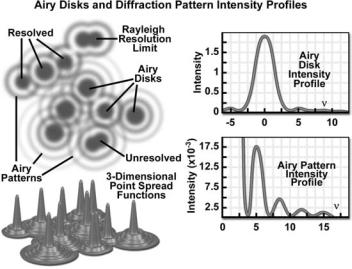
Imaging a point-like light source in the microscope produces an electromagnetic field in the image plane whose amplitude fluctuations can be regarded as a manifestation of the response of the optical system to the specimen. This field is commonly represented through the amplitude point spread function, and allows evaluation of the optical transfer properties of the combined system components (29,86–88). Although variations in field amplitude are not directly observable, the visible image of the point source formed in the microscope and recorded by its imaging system is the intensity point spread function, which describes the system response in real space. Actual specimens are not point sources, but can be regarded as a superposition of an infinite number of objects having dimensions below the resolution of the system. The properties of the intensity point spread function (PSF; see Fig. 12) in the image plane as well as in the axial direction are major factors in determining the resolution of a microscope (1,24,29,40,85–89).

It is possible to experimentally measure the intensity point spread function in the microscope by recording the image of a subresolution spherical bead as it is scanned through focus (a number of examples may be found in the literature). Because of the technical difficulty posed in direct measurement of the intensity point spread function, calculated point spread functions are commonly utilized to evaluate the resolution performance of different optical systems, as well as the optical-sectioning capabilities of confocal, two-photon, and conventional widefield microscopes. Although the intensity point spread function extends in all three dimensions, with regard to the relationship between resolution and contrast, it is useful to consider only the lateral components of the intensity distribution, with reference to the familiar Airy disk (24).

The intensity distribution of the point-spread function in the plane of focus is described by the rotationally symmetric Airy pattern. Because of the cylindrical symmetry of the microscope lenses, the two lateral components

(x and y) of the Airy pattern are equivalent, and the pattern represents the lateral intensity distribution as a function of distance from the optical axis (24). The lateral distance is normalized by the numerical aperture of the system and the wavelength of light, and therefore is dimensionless. Figure 12 (Airy disk and intensity function) illustrates diagrammatically the formation and characteristics of the Airy disk, the related 3D point spread function, and Airy patterns in the fluorescence microscope. Following the excitation of fluorophores in a point-like specimen region, fluorescence emission occurs in all directions, a small fraction of which is selected and focused by the optical components into an image plane where it forms an Airy disk surrounded by concentric rings of successively decreasing maximum and minimum intensity (the Airy pattern). The Airy pattern intensity distribution is the result of Fraunhofer diffraction of light passing through a circular aperture, and in a perfect optical system exhibits a central intensity maximum and higher order maxima separated by regions of zero intensity (85). The distance of the zero crossings from the optical axis, when the distance is normalized by the numerical aperture and wavelength, occur periodically (Fig. 12). When the intensity on the optical axis is normalized to one (100%), the proportional heights of the first four higher order maxima are 1.7%, 0.4%, 0.2%, and 0.08%, respectively.

A useful approach to the concept of resolution is based on consideration of an image formed by two point-like objects (specimen features), under the assumption that the image-forming process is incoherent, and that the interaction of the separate object images can be described using intensity point spread functions. The resulting image is then composed of the sum of two Airy disks, the characteristics of which depend on the separation distance between the two points (24,86). When sufficiently separated, the intensity change in the area between the objects is the maximum possible, cycling from the peak intensity (at the first point) to zero and returning to the maximum value at the center of the second point. At decreased distance in object space, the intensity distribution functions of the two points, in the image plane, begin to overlap and the resulting image may appear to be that of a single larger or brighter object or feature rather than being recognizable as two objects. If resolution is defined, in general terms, as the minimum separation distance at which the two objects can be sufficiently distinguished, it is obvious that this property is related to the width of the intensity peaks (the point spread function). Microscope resolution is directly related, therefore, to the full-width at half maximum (fwhm) of the instrument’s intensity point spread function in the component directions (29,86,87).

Some ambiguity in use of the term resolution results from the variability in defining the degree of separation between features and their point spread functions that is sufficient to allow them to be distinguished as two objects rather than one. In general, minute features of interest in microscopy specimens produce point images that overlap to some extent, displaying two peaks separated by a gap (1,24,29,40,86). The greater the depth of the gap between the peaks, the easier it is to distinguish, or resolve, the two

objects. By specifying the depth of the dip in intensity between two overlapping point spread functions, the ambiguity in evaluating resolution can be removed, and a quantitative aspect introduced.

In order to quantify resolution, the concept of contrast is employed, which is defined for two objects of equal intensity as the difference between their maximum intensity and the minimum intensity occurring in the space between them (55,86,89). Because the maximum intensity of the Airy disk is normalized to one, the highest achievable contrast is also one, and occurs only when the spacing between the two objects is relatively large, with sufficient separation to allow the first zero crossing to occur in their combined intensity distribution. At decreased distance, as the two point spread functions begin to overlap, the dip in intensity between the two maxima (and the contrast) is increasingly reduced. The distance at which two peak maxima are no longer discernible, and the contrast becomes zero, is referred to as the contrast cut-off distance (24,40). The variation of contrast with distance allows resolution, in terms of the separation of two points, to be defined as a function of contrast.

The relationship between contrast and separation distance for two point-like objects is referred to as the contrast/distance function or contrast transfer function (31,90). Resolution can be defined as the separation distance at which two objects are imaged with a certain contrast value. It is obvious that when zero contrast exists, the points are not resolved; the so-called Sparrow criterion defines the resolution of an optical system as being equivalent to the contrast cut-off distance (24). It is common, however, to specify that greater contrast is necessary to adequately distinguish two closely spaced points visually, and the well-known Rayleigh criterion (24) for resolution states that two points are resolved when the first minimum (zero crossing) of one Airy disk is aligned with the central maximum of the second Airy disk. Under optimum imaging conditions, the Rayleigh criterion separation distance corresponds to a contrast value of 26.4%. Although any contrast value >0 can be specified in defining resolution, the 26% contrast of the Rayleigh criterion is considered reasonable in typical fluorescence microscopy applications, and is the basis for the common expression defining lateral resolution according to the following equation (24), in which the point separation (r) in the image plane is the distance between the central maximum and the first minimum in the Airy disk:

rlateral ¼ 1:22 l=ð2 NAÞ ¼ 0:6 l=NA

where l is the emitted light wavelength and NA is the numerical aperture of the objective.

Resolution in the microscope is directly related to the fwhm dimensions of the microscope’s point spread function, and it is common to measure this value experimentally in order to avoid the difficulty in attempting to identify intensity maxima in the Airy disk. Measurements of resolution utilizing the fwhm values of the point spread function are somewhat smaller than those calculated employing the Rayleigh criterion. Furthermore, in confocal fluorescence configurations, single-point illumination scanning and

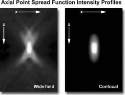
464 MICROSCOPY, CONFOCAL

single-point detection are employed, so that only the fluorophores in the shared volume of the illumination and detection point spread functions are able to be detected. The intensity point spread function in the confocal case is, therefore, the product of the independent illumination intensity and detection intensity point spread functions. For confocal fluorescence, the lateral (and axial) extent of the point spread function is reduced by 30% compared to that in the wide-field microscope. Because of the narrower intensity point spread function, the separation of points required to produce acceptable contrast in the confocal microscope (29,31) is reduced to a distance approximated by

rlateral ¼ 0:4l=NA

If the illumination and fluorescence emission wavelengths are approximately the same, the confocal fluorescence microscope Airy disk size is the square of the wide-field microscope Airy disk. Consequently, the contrast cut-off distance is reduced in the confocal arrangement, and equivalent contrast can be achieved at a shorter distance compared to the widefield illumination configuration. Regardless of the instrument configuration, the lateral resolution displays a proportional relationship to wavelength, and is inversely proportional to the objective lens numerical aperture.

As noted previously, lateral resolution is of primary interest in discussing resolution and contrast, although the axial extent of the microscope intensity point spread function is similarly reduced in the confocal arrangement as compared to the widefield fluorescence configuration (86,89). Reasonable contrast between point-like objects lying on the optical axis occurs when they are separated by the distance between the central maximum and the first minimum of the axial point spread function component.

Figure 13 presents the axial intensity distributions (89) for a typical widefield (Fig. 13a) and confocal (Fig. 13b) fluorescence microscope. Note the dramatic reduction in intensity of the wings in the confocal distribution as a function of distance from the central maximum.

A variety of equations are presented in the literature that pertains to different models for calculating axial resolution for various microscope configurations. The ones

Figure 13. Comparison of axial (x–z) point spread functions for widefield (left) and confocal (right) microscopy.

most applicable to fluorescence emission are similar in form to the expressions evaluating depth of field, and demonstrate that axial resolution is proportional to the wavelength, and refractive index of the specimen medium, and inversely proportional to the square of the numerical aperture. Consequently, the NA of the microscope objective has a much greater effect on axial resolution than does the emission wavelength. One equation (89) commonly used to describe axial resolution for the confocal configuration is given below, with h representing the index of refraction, and the other variables as specified previously:

raxial ¼ 1:4 l h=NA2

Although the confocal microscope configuration exhibits only a modest improvement in measured axial resolution over that of the widefield microscope, the true advantage of the confocal approach is in the optical sectioning capability in thick specimens, which results in a dramatic improvement in effective axial resolution over conventional techniques. The optical sectioning properties of the confocal microscope result from the characteristics of the integrated intensity point spread function, which has a maximum in the focal plane when evaluated as a function of depth. The equivalent integral of intensity point spread function for the conventional widefield microscope is constant as a function of depth, producing no optical sectioning capabilities.

FLUOROPHORES FOR CONFOCAL MICROSCOPY

Biological laser scanning confocal microscopy relies heavily on fluorescence as an imaging mode, primarily due to the high degree of sensitivity afforded by the technique coupled with the ability to specifically target structural components and dynamic processes in chemically fixed as well as living cells and tissues. Many fluorescent probes are constructed around synthetic aromatic organic chemicals designed to bind with a biological macromolecule (e.g., a protein or nucleic acid) or to localize within a specific structural region, such as the cytoskeleton, mitochondria, Golgi apparatus, endoplasmic reticulum, and nucleus (90). Other probes are employed to monitor dynamic processes and localized environmental variables, including concentrations of inorganic metallic ions, pH, reactive oxygen species, and membrane potential (91). Fluorescent dyes are also useful in monitoring cellular integrity (live versus dead and apoptosis), endocytosis, exocytosis, membrane fluidity, protein trafficking, signal transduction, and enzymatic activity (92). In addition, fluorescent probes have been widely applied to genetic mapping and chromosome analysis in the field of molecular genetics.

The history of synthetic fluorescent probes dates back over a century to the late-1800s when many of the cornerstone dyes for modern histology were developed. Among these were pararosaniline, methyl violet, malachite green, safranin O, methylene blue, and numerous azo (nitrogen) dyes, such as Bismarck brown (93). Although these dyes were highly colored and capable of absorbing selected bands of visible light, most were only weakly fluorescent and would not be useful for the fluorescence microscopes that would be developed several decades later. However,

several synthetic dye classes synthesized during this period, based on the xanthene and acridine heterocyclic ring systems, proved to be highly fluorescent and provided a foundation for the development of modern synthetic fluorescent probes. Most notable among these early fluorescent dyes were the substituted xanthenes, fluorescein and rhodamine B, and the biaminated acridine derivative, acridine orange.

Fluorochromes were introduced to fluorescence microscopy in the early twentieth century as vital stains for bacteria, protozoa, and trypanosomes, but did not see widespread use until the 1920s when fluorescence microscopy was first used to study dye binding in fixed tissues and living cells (7,93). However, it was not until the early 1940s that Coons developed a technique for labeling antibodies with fluorescent dyes, thus giving birth to the field of immunofluorescence (94). Over the past 60 years, advances in immunology and molecular biology have produced a wide spectrum of secondary antibodies and provided insight into the molecular design of fluorescent probes targeted at specific regions within macromolecular complexes.

Fluorescent probe technology and cell biology were dramatically altered by the discovery of the GFP from jellyfish and the development of mutant spectral variants, which have opened the door to noninvasive fluorescence multicolor investigations of subcellular protein localization, intermolecular interactions, and trafficking using living cell cultures (79,80,95). More recently, the development of nanometer-sized fluorescent semiconductor quantum dots has provided a new avenue for research in confocal and widefield fluorescence microscopy (96). Despite the numerous advances made in fluorescent dye synthesis during the past few decades, there is very little solid evidence about molecular design rules for developing new fluorochromes, particularly with regard to matching absorption spectra to available confocal laser excitation wavelengths. As a result, the number of fluorophores that have found widespread use in confocal microscopy is a limited subset of the many thousands that have been discovered.

BASIC CHARACTERISTICS OF FLUOROPHORES

Fluorophores are catalogued and described according to their absorption and fluorescence properties, including the spectral profiles, wavelengths of maximum absorbance and emission, and the fluorescence intensity of the emitted light (92). One of the most useful quantitative parameters for characterizing absorption spectra is the molar extinction coefficient (denoted with the Greek symbole, see Fig. 14a), which is a direct measure of the ability of a molecule to absorb light. The extinction coefficient is useful for converting units of absorbance into units of molar concentration, and is determined by measuring the absorbance at a reference wavelength (usually the maximum, characteristic of the absorbing species) for a molar concentration in a defined optical path length. The quantum yield of a fluorochrome or fluorophore represents a quantitative measure of fluorescence emission efficiency, and is expressed as the ratio of the number of photons emitted to the number of photons absorbed. In other words, the quantum

Figure 14. Fluorescent spectral profiles, plotted as normalized absorption or emission as a function of wavelength, for popular synthetic fluorophores emitting in the blue, green, and red regions of the visible spectrum. Each profile is identified with a colored bullet in (a), which illustrates excitation spectra. (b) The emission spectra for the fluorophores according to the legend in (a).

yield represents the probability that a given excited fluorochrome will produce an emitted (fluorescence) photon. Quantum yields typically range between a value of 0 and 1 and fluorescent molecules commonly employed as probes in microscopy have quantum yields ranging from very low (0.05 or less) to almost unity. In general, a high quantum yield is desirable in most imaging applications. The quantum yield of a given fluorophore varies, sometimes to large extremes, with environmental factors, such as metallic ion concentration, pH, and solvent polarity (92).

In most cases, the molar extinction coefficient for photon absorption is quantitatively measured and expressed at a specific wavelength, whereas the quantum efficiency is an assessment of the total integrated photon emission over the entire spectral band of the fluorophore (Fig. 14b). As opposed to traditional arc-discharge lamps used with the shortest range (10–20 nm) bandpass interference filters in wide-field fluorescence microscopy, the laser systems used for fluorophore excitation in scanning confocal microscopy restrict excitation to specific laser spectral lines that encompass only a few nanometers (1,7). The fluorescence emission spectrum for both techniques, however, is controlled by similar bandpass or longpass filters that can cover tens to hundreds of nanometers (7). Below saturation levels, fluorescence intensity is proportional to the product of the molar extinction coefficient and the quantum yield of the fluorophore, a relationship that can be utilized to judge the effectiveness of emission as a function of excitation wavelength(s). These parameters display an approximate 20-fold range in variation for the popular fluorophores commonly employed for investigations in confocal microscopy with quantum yields ranging from 0.05 to 1.0, and extinction coefficients ranging from 10,000 to 0.25 million (L mol 1). In general, the absorption spectrum of a fluorophore is far less dependent on environmental conditions than the fluorescence emission characteristics (spectral wavelength profile and quantum yield; 92).

Fluorophores chosen for confocal applications must exhibit a brightness level and signal persistence sufficient for the instrument to obtain image data that does not suffer from excessive photobleaching artifacts and low signal/ noise ratios. In widefield fluorescence microscopy, excitation illumination levels are easily controlled with neutral

density filters (40), and the intensity can be reduced (coupled with longer emission signal collection periods) to avoid saturation and curtail irreversible loss of fluorescence. Excitation conditions in confocal microscopy are several orders of magnitude more severe, however, and restrictions imposed by characteristics of the fluorophores and efficiency of the microscope optical system become the dominating factor in determining excitation rate and emission collection strategies (1,7,92).

Because of the narrow and wavelength-restricted laser spectral lines employed to excite fluorophores in confocal microscopy (Table 1), fluorescence emission intensity can be seriously restricted due to poor overlap of the excitation wavelengths with the fluorophore absorption band. In addition, the confocal pinhole aperture, which is critical in obtaining thin optical sections at high signal/noise ratios, is responsible for a 25–50% loss of emission intensity, regardless of how much effort has been expended on fine-tuning and alignment of the microscope optical system

(7). Photomultiplier tubes are the most common detectors in confocal microscopy, but suffer from a quantum efficiency that varies as a function of wavelength (especially in the red and IR regions), further contributing to a wave- length-dependent loss of signal across the emission spectrum (59–62). Collectively, the light losses in confocal microscopy can result in a reduction of intensity exceeding 50 times of the level typically observed in widefield fluorescence instruments. It should be clear from the preceding argument that fluorophore selection is one of the most critical aspects of confocal microscopy, and instrumental efficiency must be carefully considered, as well, in order to produce high quality images.

In confocal microscopy, irradiation of the fluorophores with a focused laser beam at high power densities increases the emission intensity up to the point of dye saturation, a condition whose parameters are dictated by the excited state lifetime (97). In the excited state, fluorophores are unable to absorb another incident photon until they emit a lower energy photon through the fluorescence process. When the rate of fluorophore excitation exceeds the rate of emission decay, the molecules become saturated and the ground state population decreases. As a result, a majority of the laser energy passes through the specimen undiminished and does not contribute to fluorophore excitation. Balancing fluorophore saturation with laser light intensity

levels is, therefore, a critical condition for achieving the optimal signal/noise ratio in confocal experiments (1,7,92,97). The number of fluorescent probes currently available for confocal microscopy runs in the hundreds (90,93), with many dyes having absorption maxima closely associated with common laser spectral lines (90). An exact match between a particular laser line and the absorption maximum of a specific probe is not always possible, but the excitation efficiency of lines near the maximum is usually sufficient to produce a level of fluorescence emission that can be readily detected.

Instrumentally, fluorescence emission collection can be optimized by careful selection of objectives, detector aperture dimensions, dichromatic and barrier filters, as well as maintaining the optical train in precise alignment (63). In most cases, low magnification objectives with a high numerical aperture should be chosen for the most demanding imaging conditions because light collection intensity increases as the fourth power of the numerical aperture, but only decreases as the square of the magnification. However, the most important limitations in light collection efficiency in confocal microscopy arise from restrictions imposed by the physical properties of the fluorophores themselves. As previously discussed, fluorescent probe development is limited by a lack of knowledge of the specific molecular properties responsible for producing optimum fluorescence characteristics, and the design rules are insufficiently understood to be helpful as a guide to the development of more efficient fluorophores. The current success in development of new fluorescent probes capable of satisfactory performance in confocal microscopy is a testament to the progress made through use of empirical data and assumptions about molecular structure extrapolated from the properties of existing dyes, many of which were first synthesized over a hundred years ago.

TRADITIONAL FLUORESCENT DYES

The choice of fluorescent probes for confocal microscopy must address the specific capabilities of the instrument to excite and detect fluorescence emission in the wavelength regions made available by the laser systems and detectors. Although the current lasers used in confocal microscopy (Table 1) produce discrete lines in the UV, visible, and

near-IR portions of the spectrum, the location of these spectral lines does not always coincide with absorption maxima of popular fluorophores. In fact, it is not necessary for the laser spectral line to correspond exactly with the fluorophore wavelength of maximum absorption, but the intensity of fluorescence emission is regulated by the fluorophore extinction coefficient at the excitation wavelength (as discussed above). The most popular lasers for confocal microscopy are air-cooled argon and krypton–argon ion lasers, the new blue diode lasers, and a variety of helium– neon systems (7,40). Collectively, these lasers are capable of providing excitation at 10–12 specific wavelengths between 400 and 650 nm.

Many of the classical fluorescent probes that have been successfully utilized for many years in widefield fluorescence (92,93), including fluorescein isothiocyanate, Lissamine rhodamine, and Texas red, are also useful in confocal microscopy. Fluorescein is one of the most popular fluorochromes ever designed, and has enjoyed extensive application in immunofluorescence labeling. This xanthene dye has an absorption maximum at 495 nm, which coincides quite well with the 488 nm (blue) spectral line produced by argon-ion and krypton–argon lasers, as well as the 436 and 467 principal lines of the mercury and xenon arc-discharge lamps, respectively. In addition, the quantum yield of fluorescein is very high and a significant amount of information has been gathered on the characteristics of this dye with respect to the physical and chemical properties (98). On the negative side, the fluorescence emission intensity of fluorescein is heavily influenced by environmental factors (e.g., pH), and the relatively broad emission spectrum often overlaps with those of other fluorophores in dual and triple labeling experiments (92,98,99).

Tetramethyl rhodamine (TMR) and the isothiocyanate derivative (TRITC) are frequently employed in multiple labeling investigations in widefield microscopy due to their efficient excitation by the 546 nm spectral line from mercury arc-discharge lamps. The fluorochromes, which have significant emission spectral overlap with fluorescein, can be excited very effectively by the 543 nm line from helium–neon lasers, but not by the 514 or 568 nanometer lines from argon-ion and krypton–argon lasers (99). When using krypton-based laser systems, Lissamine rhodamine is a far better choice in this fluorochrome class due to the absorption maximum at 575 nm and its spectral separation from fluorescein. Also, the fluorescence emission intensity of rhodamine derivatives is not as dependent upon strict environmental conditions as that of fluorescein.

Several of the acridine dyes, first isolated in the nineteenth century, are useful as fluorescent probes in confocal microscopy (93). The most widely utilized, acridine orange, consists of the basic acridine nucleus with dimethylamino substituents located at the 3 and 6 positions of the trinuclear ring system. In physiological pH ranges, the molecule is protonated at the heterocyclic nitrogen and exists predominantly as a cationic species in solution. Acridine orange binds strongly to DNA by intercalation of the acridine nucleus between successive base pairs, and exhibits green fluorescence with a maximum wavelength of 530 nm (92,93,100). The probe also binds strongly to ribonucleic acid (RNA) or single-stranded deoxyribonucleic

acid (DNA), but has a longer wavelength fluorescence maximum ( 640 nm; red) when bound to these macromolecules. In living cells, acridine orange diffuses across the cell membrane (by virtue of the association constant for protonation) and accumulates in the lysosomes and other acidic vesicles. Similar to most acridines and related polynuclear nitrogen heterocycles, acridine orange has a relatively broad absorption spectrum, which enables the probe to be used with several wavelengths from the argon-ion laser.

Another popular traditional probe that is useful in confocal microscopy is the phenanthridine derivative, propidium iodide, first synthesized as an antitrypanosomal agent along with the closely related ethidium bromide). Propidium iodide binds to DNA in a manner similar to the acridines (via intercalation) to produce orange-red fluorescence centered at 617 nm (101,102). The positively charged fluorophore also has a high affinity for doublestranded RNA. Propidium has an absorption maximum at 536 nm, and can be excited by the 488 or 514-nm spectral lines of an argon-ion (or krypton–argon) laser, or the 543 nm line from a green helium–neon laser. The dye is often employed as a counterstain to highlight cell nuclei during double or triple labeling of multiple intracellular structures. Environmental factors can affect the fluorescence spectrum of propidium, especially when the dye is used with mounting media containing glycerol. The structurally similar ethidium bromide, which also binds to DNA by intercalation (102), produces more background staining, and is therefore not as effective as propidium.

The DNA and chromatin can also be stained with dyes that bind externally to the double helix. The most popular fluorochromes in this category are 40,6-diamidino-2-pheny- lindole (DAPI) and the bis (benzimide) Hoechst dyes that are designated by the numbers 33258, 33342, and 34580 (103–106). These probes are quite water soluble and bind externally to AT-rich base pair clusters in the minor groove of double-stranded DNA with a dramatic increase in fluorescence intensity. Both dye classes can be stimulated by the 351 nm spectral line of high power argon-ion lasers or the 354 nm line from a helium–cadmium laser. Similar to the acridines and phenanthridines, these fluorescent probes are popular choices as a nuclear counterstain for use in multicolor fluorescent labeling protocols. The vivid blue fluorescence emission produces dramatic contrast when coupled to green, yellow, and red probes in adjacent cellular structures.

ALEXA FLUOR DYES

The dramatic advances in modern fluorophore technology are exemplified by the Alexa Fluor dyes (90,107,108) introduced by Molecular Probes (Alexa Fluor is a registered trademark of Molecular Probes). These sulfonated rhodamine derivatives exhibit higher quantum yields for more intense fluorescence emission than spectrally similar probes, and have several additional improved features, including enhanced photostability, absorption spectra matched to common laser lines, pH insensitivity, and a high degree of water solubility. In fact, the resistance to photobleaching of Alexa Fluor dyes is so dramatic (108)

468 MICROSCOPY, CONFOCAL

that even when subjected to irradiation by high intensity laser sources, fluorescence intensity remains stable for relatively long periods of time in the absence of antifade reagents. This feature enables the water soluble Alexa Fluor probes to be readily utilized for both live-cell and tissue section investigations, as well as in traditional fixed preparations.

Alexa Fluor dyes are available in a broad range of fluorescence excitation and emission wavelength maxima, ranging from the UV and deep blue to the near-IR regions (90). Alphanumeric names of the individual dyes are associated with the specific excitation laser or arc-discharge lamp spectral lines for which the probes are intended. For example, Alexa Fluor 488 is designed for excitation by the blue 488 nm line of the argon or krypton–argon ion lasers, while Alexa Fluor 568 is matched to the 568 nm spectral line of the krypton–argon laser. Several of the Alexa Fluor dyes are specifically designed for excitation by either the blue diode laser (405 nm), the orange/yellow helium–neon laser (594 nm), or the red helium–neon laser (633 nm). Other Alexa Fluor dyes are intended for excitation with traditional mercury arc-discharge lamps in the visible (Alexa Fluor 546) or UV (Alexa Fluor 350, also useful with high power argon-ion lasers), and solid-state red diode lasers (Alexa Fluor 680). Because of the large number of available excitation and emission wavelengths in the Alexa Fluor series, multiple labeling experiments can often be conducted exclusively with these dyes.

Alexa Fluor dyes are commercially available as reactive intermediates in the form of maleimides, succinimidyl esters, and hydrazides, as well as prepared cytoskeletal probes (conjugated to phalloidin, G-actin, and rabbit skeletal muscle actin) and conjugates to lectin, dextrin, streptavidin, avidin, biocytin, and a wide variety of secondary antibodies (90). In the latter forms, the Alexa Fluor fluorophores provide a broad palette of tools for investigations in immunocytochemistry, neuroscience, and cellular biology. The family of probes has also been extended into a series of dyes having overlapping fluorescence emission maxima targeted at sophisticated confocal microscopy detection systems with spectral imaging and linear unmixing capabilities. For example, Alexa Fluor 488, Alexa Fluor 500, and Alexa Fluor 514 are visually similar in color with bright green fluorescence, but have spectrally distinct emission profiles. In addition, the three fluorochromes can be excited with the 488 or 514 nm spectral line from an argon-ion laser and are easily detected with traditional fluorescein filter combinations. In multispectral (x–y–l; referred to as a lambda stack) confocal imaging experiments, optical separation software can be employed to differentiate between the similar signals (32–35). The overlapping emission spectra of Alexa Fluor 488, 500, and 514 are segregated into separate channels and differentiated using pseudocolor techniques when the three fluorophores are simultaneously combined in a triple label investigation.

CYANINE DYES

The popular family of cyanine dyes, Cy2, Cy3, Cy5, Cy7, and their derivatives, are based on the partially saturated

indole nitrogen heterocyclic nucleus with two aromatic units being connected via a polyalkene bridge of varying carbon number (92,109). These probes exhibit fluorescence excitation and emission profiles that are similar to many of the traditional dyes, such as fluorescein and tetramethylrhodamine, but with enhanced water solubility, photostability, and higher quantum yields. Most of the cyanine dyes are more environmentally stable than their traditional counterparts, rendering their fluorescence emission intensity less sensitive to pH and organic mounting media. In a manner similar to the Alexa Fluors, the excitation wavelengths of the Cy series of synthetic dyes are tuned specifically for use with common laser and arc-discharge sources, and the fluorescence emission can be detected with traditional filter combinations.

Marketed by a number of distributors, the cyanine dyes are readily available as reactive dyes or fluorophores coupled to a wide variety of secondary antibodies, dextrin, streptavidin, and eggwhite avidin (110). The cyanine dyes generally have broader absorption spectral regions than members of the Alexa Fluor family, making them somewhat more versatile in the choice of laser excitation sources for confocal microscopy (7). For example, using the 547 nm spectral line from an argon-ion laser, Cy2 is about twice as efficient in fluorescence emission as Alexa Fluor 488. In an analogous manner, the 514 nm argon-ion laser line excites Cy3 with a much higher efficiency than Alexa Fluor 546, a spectrally similar probe. Emission profiles of the cyanine dyes are comparable in spectral width to the Alexa Fluor series.

Included in the cyanine dye series are the long-wave- length Cy5 derivatives, which are excited in the red region (650 nm) and emit in the far-red (680 nm) wavelengths. The Cy5 fluorophore is very efficiently excited by the 647 nm spectral line of the krypton–argon laser, the 633 nm line of the red helium–neon laser, or the 650 nm line of the red diode laser, providing versatility in laser choice. Because the emission spectral profile is significantly removed from traditional fluorophores excited by UV and blue illumination, Cy5 is often utilized as a third fluorophore in triple labeling experiments. However, similar to other probes with fluorescence emission in the far-red spectral region, Cy5 is not visible to the human eye and can only be detected electronically (using a specialized CCD camera system or photomultiplier). Therefore, the probe is seldom used in conventional widefield fluorescence experiments.

FLUORESCENT ENVIRONMENTAL PROBES

Fluorophores designed to probe the internal environment of living cells have been widely examined by a number of investigators, and many hundreds have been developed to monitor such effects as localized concentrations of alkali and alkaline earth metals, heavy metals (employed biochemically as enzyme cofactors), inorganic ions, thiols, and sulfides, nitrite, as well as pH, solvent polarity, and membrane potential (7,90–93,111,112). Originally, the experiments in this arena were focused on changes in the wavelength and/or intensity of absorption and emission spectra exhibited by fluorophores upon binding calcium

ions in order to measure intracellular flux densities. These probes bind to the target ion with a high degree of specificity to produce the measured response and are often referred to as spectrally sensitive indicators. Ionic concentration changes are determined by the application of optical ratio signal analysis to monitor the association equilibrium between the ion and its host. The concentration values derived from this technique are largely independent of instrumental variations and probe concentration fluctuations due to photobleaching, loading parameters, and cell retention. In the past few years, a number of new agents have been developed that bind specific ions or respond with measurable features to other environmental conditions (7,90).

Calcium is a metabolically important ion that plays a vital role in cellular response to many forms of external stimuli (113). Because transient fluctuations in calcium ion concentration are typically involved when cells undergo a response, fluorophores must be designed to measure not only localized concentrations within segregated compartments, but should also produce quantitative changes when flux density waves progress throughout the entire cytoplasm. Many of the synthetic molecules designed to measure calcium levels are based on the nonfluorescent chelation agents EGTA and BAPTA, which have been used for years to sequester calcium ions in buffer solutions (7,114,115). Two of the most common calcium probes are the ratiometric indicators fura-2 and indo-1, but these fluorophores are not particularly useful in confocal microscopy (7,116). The dyes are excited by UV light and exhibit a shift in the excitation or emission spectrum with the formation of isosbestic points when binding calcium. However, the optical aberrations associated with UV imaging, limited specimen penetration depths, and the expense of ultraviolet lasers have limited the utility of these probes in confocal microscopy.

Fluorophores that respond in the visible range to calcium ion fluxes are, unfortunately, not ratiometric indicators and do not exhibit a wavelength shift (typical of fura-2 and indo-1) upon binding, although they do undergo an increase or decrease in fluorescence intensity. The best example is fluo-3, a complex xanthene derivative, which undergoes a dramatic increase in fluorescence emission at 525 nm (green) when excited by the 488 nm spectral line of an argon-ion or krypton–argon laser (7,117). Because isosbestic points are not present to assure the absence of concentration fluctuations, it is impossible to determine whether spectral changes are due to complex formation or a variation in concentration with fluo-3 and similar fluorophores.

To overcome the problems associated with using visible light probes lacking wavelength shifts (and isosbestic points), several of these dyes are often utilized in combination for calcium measurements in confocal microscopy (118). Fura red, a multinuclear imidazole and benzofuran heterocycle, exhibits a decrease in fluorescence at 650 nm when binding calcium. A ratiometric response to calcium ion fluxes can be obtained when a mixture of fluo-3 and fura red is excited at 488 nm and fluorescence is measured at the emission maxima (525 and 650 nm, respectively) of the two probes. Because the emission intensity of fluo-3 increases monotonically while that of fura red simultaneously

decreases, an isosbestic point is obtained when the dye concentrations are constant within the localized area being investigated. Another benefit of using these probes together is the ability to measure fluorescence intensity fluctuations with a standard FITC/Texas red interference filter combination.

Quantitative measurements of ions other than calcium, such as magnesium, sodium, potassium, and zinc, are conducted in an analogous manner using similar fluorophores (7,90,92). One of the most popular probes for magnesium, mag-fura-2 (structurally similar to fura red), is also excited in the ultraviolet range and presents the same problems in confocal microscopy as fura-2 and indo-1. Fluorophores excited in the visible light region are becoming available for the analysis of many monovalent and divalent cations that exist at varying concentrations in the cellular matrix. Several synthetic organic probes have also been developed for monitoring the concentration of simple and complex anions.

Important fluorescence monitors for intracellular pH include a pyrene derivative known as HPTS or pyranine, the fluorescein derivative, BCECF, and another substituted xanthene termed carboxy SNARF-1 (90,119–122). Because many common fluorophores are sensitive to pH in the surrounding medium, changes in fluorescence intensity that are often attributed to biological interactions may actually occur as a result of protonation. In the physiological pH range (pH 6.8–7.4), the probes mentioned above are useful for dual-wavelength ratiometric measurements and differ only in dye loading parameters. Simultaneous measurements of calcium ion concentration and pH can often be accomplished by combining a pH indicator, such as SNARF- 1, with a calcium ion indicator (e.g., fura-2). Other probes have been developed for pH measurements in subcellular compartments, such as the lysosomes, as described below.

ORGANELLE PROBES

Fluorophores targeted at specific intracellular organelles, such as the mitochondria, lysosomes, Golgi apparatus, and endoplasmic reticulum, are useful for monitoring a variety of biological processes in living cells using confocal microscopy (7,90,92). In general, organelle probes consist of a fluorochrome nucleus attached to a target-specific moiety that assists in localizing the fluorophore through covalent, electrostatic, hydrophobic, or similar types of bonds. Many of the fluorescent probes designed for selecting organelles are able to permeate or sequester within the cell membrane (and therefore, are useful in living cells), while others must be installed using monoclonal antibodies with traditional immunocytochemistry techniques. In living cells, organelle probes are useful for investigating transport, respiration, mitosis, apoptosis, protein degradation, acidic compartments, and membrane phenomena. Cell impermeant fluorophore applications include nuclear functions, cytoskeletal structure, organelle detection, and probes for membrane integrity. In many cases, living cells that have been labeled with permeant probes can subsequently be fixed and counterstained with additional fluorophores in multicolor labeling experiments.

470 MICROSCOPY, CONFOCAL

Mitochondrial probes are among the most useful fluorophores for investigating cellular respiration and are often employed along with other dyes in multiple labeling investigations. The traditional probes, rhodamine 123 and tetramethylrosamine, are rapidly lost when cells are fixed and have largely been supplanted by newer, more specific, fluorophores developed by Molecular Probes (90,123,124). These include the popular MitoTracker and MitoFluor series of structurally diverse xanthene, benzoxazole, indole, and benzimidazole heterocycles that are available in a variety of excitation and emission spectral profiles. The mechanism of action varies for each of the probes in this series, ranging from covalent attachment to oxidation within respiring mitochondrial membranes.

MitoTracker dyes are retained quite well after cell fixation in formaldehyde and can often withstand lipophilic permeabilizing agents (123). In contrast, the MitoFluor probes are designed specifically for actively respiring cells and are not suitable for fixation and counterstaining procedures (90). Another popular mitochondrial probe, entitled JC-1, is useful as an indicator of membrane potential and in multiple staining experiments with fixed cells (125). This carbocyanine dye exhibits green fluorescence at low concentrations, but can undergo intramolecular association within active mitochondria to produce a shift in emission to longer (red) wavelengths. The change in emission wavelength is useful in determining the ratio of active to nonactive mitochondria in living cells.

In general, weakly basic amines that are able to pass through membranes are the ideal candidates for investigating biosynthesis and pathogenesis in lysosomes (90–92,112). Traditional lysosomal probes include the nonspecific phenazine and acridine derivatives neutral red and acridine orange, which are accumulated in the acidic vesicles upon being protonated (92,93). Fluorescently labeled latex beads and macromolecules, such as dextran, can also be accumulated in lysosomes by endocytosis for a variety of experiments. However, the most useful tools for investigating lysosomal properties with confocal microscopy are the LysoTracker and LysoSensor dyes developed by Molecular Probes (90,92,126). These structurally diverse agents contain heterocyclic and aliphatic nitrogen moieties that modulate transport of the dyes into the lysosomes of living cells for both shortand long-term studies. The LysoTracker probes, which are available in a variety of excitation and emission wavelengths (91), have high selectivity for acidic organelles and are capable of labeling cells at nanomolar concentrations. Several of the dyes are retained quite well after fixing and permeabilization of cells. In contrast, the LysoSensor fluorophores are designed for studying dynamic aspects of lysosome function in living cells. Fluorescence intensity dramatically increases in the LysoSensor series upon protonation, making these dyes useful as pH indicators (91). A variety of Golgi apparatus specific monoclonal antibodies have also been developed for use in immunocytochemistry assays (90,127–129).

Proteins and lipids are sorted and processed in the Golgi apparatus, which is typically stained with fluorescent derivatives of ceramides and sphingolipids (130). These agents are highly lipophilic, and are therefore useful as markers for the study of lipid transport and metabolism in

live cells. Several of the most useful fluorophores for Golgi apparatus contain the complex heterocyclic BODIPY nucleus developed by Molecular Probes (90,92,131). When coupled to sphingolipids, the BODIPY fluorophore is highly selective and exhibits a tolerance for photobleaching that is far superior to many other dyes. In addition, the emission spectrum is dependent upon concentration (shifting from green to red at higher concentrations), making the probes useful for locating and identifying intracellular structures that accumulate large quantities of lipids. During live-cell experiments, fluorescent lipid probes can undergo metabolism to derivatives that may bind to other subcellular features, a factor that can often complicate the analysis of experimental data.

The most popular traditional probes for endoplasmic reticulum fluorescence analysis are the carbocyanine and xanthene dyes, DiOC (6) and several rhodamine derivatives, respectively (90,92). These dyes must be used with caution, however, because they can also accumulate in the mitochondria, Golgi apparatus, and other intracellular lipophilic regions. Newer, more photostable, probes have been developed for selective staining of the endoplasmic reticulum by several manufacturers. In particular, oxazole members of the Dapoxyl family produced by Molecular Probes are excellent agents for selective labeling of the endoplasmic reticulum in living cells, either alone or in combination with other dyes (90). These probes are retained after fixation with formaldehyde, but can be lost with permeabilizing detergents. Another useful probe is Brefeldin A (131), a stereochemically complex fungal metabolite that serves as an inhibitor of protein trafficking out of the endoplasmic reticulum. Finally, similar to other organelles, monoclonal antibodies (127–129) have been developed that target the endoplasmic reticulum in fixed cells for immunocytochemistry investigations.

QUANTUM DOTS

Nanometer-sized crystals of purified semiconductors known as quantum dots are emerging as a potentially useful fluorescent labeling agent for living and fixed cells in both traditional widefield and laser scanning confocal fluorescence microscopy (132–136). Recently introduced techniques enable the purified tiny semiconductor crystals to be coated with a hydrophilic polymer shell and conjugated to antibodies or other biologically active peptides and carbohydrates for application in many of the classical immunocytochemistry protocols (Fig. 15). These probes have significant benefits over organic dyes and fluorescent proteins, including long-term photostability, high fluorescence intensity levels, and multiple colors with singlewavelength excitation for all emission profiles (136).

Quantum dots produce illumination in a manner similar to the well-known semiconductor light emitting diodes, but are activated by absorption of a photon rather than an electrical stimulus. The absorbed photon creates an elec- tron-hole pair that quickly recombines with the concurrent emission of a photon having lower energy. The most useful semiconductor discovered thus far for producing biological quantum dots is cadmium selenide (CdSe), a material in

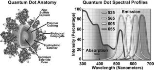
Figure 15. Anatomy and spectral profiles of quantum dot conjugates. The cadmium selenide core is encapsulated with zinc sulfide, and then a polymer coating is applied followed by a hydrophilic exterior to which the biological conjugate is attached (left). The absorption profile displays a shoulder at 400 nm, while the emission spectra all feature similar symmetrical profiles.

which the energy of the emitted photons is a function of the physical size of the nanocrystal particles. Thus, quantum dots having sizes that differ only by tenths of a nanometer emit different wavelengths of light, with the smaller sizes emitting shorter wavelengths, and vice versa.

Unlike typical organic fluorophores or fluorescent proteins, which display highly defined spectral profiles, quantum dots have an absorption spectrum that increases steadily with decreasing wavelength (Fig. 15). Also, in contrast, the fluorescence emission intensity is confined to a symmetrical peak with a maximum wavelength that is dependent on the dot size, but independent of the excitation wavelength (135). As a result, the same emission profile is observed regardless of whether the quantum dot is excited at 300, 400, 500, or 600 nm, but the fluorescence intensity increases dramatically at shorter excitation wavelengths. For example, the extinction coefficient for a typical quantum dot conjugate that emits in the orange region (605 nm) is approximately five-fold higher when the semiconductor is excited at 400 versus 600 nm. The fwhm value for a typical quantum dot conjugate is 30 nm (135), and the spectral profile is not skewed towards the longer wavelengths (having higher intensity tails), such is the case with most organic fluorochromes. The narrow emission profile enables several quantum dot conjugates to be simultaneously observed with a minimal level of bleed through.

For biological applications, a relatively uniform population of cadmium selenide crystals is covered with a surrounding semiconductor shell composed of zinc sulfide to improve the optical properties. Next, the core material is coated with a polymeric film and other ligands to decrease hydrophobicity and to improve the attachment efficiency of conjugated macromolecules. The final product is a biologically active particle that ranges in size from 10 to 15 nm, somewhere in the vicinity of a large protein (133). Quantum dot conjugates are solubilized as a colloidal suspension in common biological buffers and may be incorporated into existing labeling protocols in place of classical staining reagents (such as organic fluorochrome-labeled secondary antibodies).

In confocal microscopy, quantum dots are excited with varying degrees of efficiency by most of the spectral lines produced by the common laser systems, including the

argon-ion, helium–cadmium, krypton–argon, and the green helium–neon. Particularly effective at exciting quantum dots in the UV and violet regions are the new blue diode and diode-pumped solid-state lasers that have prominent spectral lines at 442 nm and below (135,136). The 405 nm blue diode laser is an economical excitation source that is very effective for use with quantum dots due to their high extinction coefficient at this wavelength. Another advantage of using these fluorophores in confocal microscopy is the ability to stimulate multiple quantum dot sizes (and spectral colors) in the same specimen with a single excitation wavelength, making these probes excellent candidates for multiple labeling experiments (137).

The exceptional photostability of quantum dot conjugates is of great advantage in confocal microscopy when optical sections are being collected. Unlike the case of organic fluorophores, labeled structures situated away from the focal plane do not suffer from excessive photobleaching during repeated raster scanning of the specimen and yield more accurate 3D volume models. In widefield fluorescence microscopy, quantum dot conjugates are available for use with conventional dye-optimized filter combinations that are standard equipment on many microscopes. Excitation can be further enhanced by substituting a shortpass filter for the bandpass filter that accompanies most filter sets, thus optimizing the amount of lamp energy that can be utilized to excite the quantum dots. Several of the custom fluorescence filter manufacturers offer combinations specifically designed to be used with quantum dot conjugates.

FLUORESCENT PROTEINS

Over the past few years, the discovery and development of naturally occurring fluorescent proteins and mutated derivatives have rapidly advanced to center stage in the investigation of a wide spectrum of intracellular processes in living organisms (75,78,80). These biological probes have provided scientists with the ability to visualize, monitor, and track individual molecules with high spatial and temporal resolution in both steady-state and kinetic experiments. A variety of marine organisms have been the source of >100 fluorescent proteins and their analogs, which arm the investigator with a balanced palette of noninvasive biological probes for single, dual, and multispectral fluorescence analysis (75). Among the advantages of fluorescent proteins over the traditional organic and new semiconductor probes described above is their response to a wider variety of biological events and signals. Coupled with the ability to specifically target fluorescent probes in subcellular compartments, the extremely low or absent photodynamic toxicity, and the widespread compatibility with tissues and intact organisms, these biological macromolecules offer an exciting new frontier in live-cell imaging.

The first member of this series to be discovered, GFP, was isolated from the North Atlantic jellyfish, Aequorea Victoria, and found to exhibit a high degree of fluorescence without the aid of additional substrates or coenzymes (138– 142). In native green fluorescent protein, the fluorescent moiety is a tripeptide derivative of serine, tyrosine, and glycine that requires molecular oxygen for activation, but no additional cofactors or enzymes (143). Subsequent

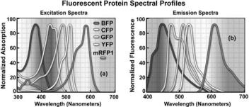
472 MICROSCOPY, CONFOCAL

investigations revealed that the GFP gene could be expressed in other organisms, including mammals, to yield fully functional analogs that display no adverse biological effects (144). In fact, fluorescent proteins can be fused to virtually any protein in living cells using recombinant complementary DNA cloning technology, and the resulting fusion protein gene product expressed in cell lines adapted to standard tissue culture methodology. Lack of a need for cell-specific activation cofactors renders the fluorescent proteins much more useful as generalized probes than other biological macromolecules, such as the phycobiliproteins, which require insertion of accessory pigments in order to produce fluorescence.

Mutagenesis experiments with green fluorescent protein have produced a large number of variants with improved folding and expression characteristics, which have eliminated wild-type dimerization artifacts and fine tuned the absorption and fluorescence properties. One of the earliest variants, known as enhanced green fluorescence protein (EGFP), contains codon substitutions (commonly referred to as the S65T mutation) that alleviates the temperature sensitivity and increases the efficiency of GFP expression in mammalian cells (145). Proteins fused with EGFP can be observed at low light intensities for long time periods with minimal photobleaching. Enhanced green fluorescent protein fusion products are optimally excited by the 488 nm spectral line from argon and krypton–argon ion lasers in confocal microscopy. This provides an excellent biological probe and instrument combination for examining intracellular protein pathways along with the structural dynamics of organelles and the cytoskeleton.

Additional mutation studies have uncovered GFP variants that exhibit a variety of absorption and emission characteristics across the entire visible spectral region, which have enabled researchers to develop probe combinations for simultaneous observation of two or more distinct fluorescent proteins in a single organism (see the spectral profiles in Fig. 16). Early investigations yielded the blue fluorescent protein (BFP) and cyan fluorescent protein (CFP) mutants from simple amino acid substitutions that shifted the absorption and emission spectral profiles of wild-type GFP to lower wavelength regions (146–148). Used in combination with GFP, these derivatives are useful in resonance energy transfer (FRET) experiments and other investigations that rely on multicolor fluorescence imaging (73). Blue fluorescent protein can be efficiently excited with the 354 nm line from a high power argon laser, while the more useful cyan derivative is excited by a number of violet and blue laser lines, including the

405 nm blue diode, the 442 nm helium–cadmium spectral line, and the 457 nm line from the standard argon-ion laser.

Another popular fluorescent protein derivative, the yellow fluorescent protein (YFP), was designed on the basis of the GFP crystalline structural analysis to red-shift the absorption and emission spectra (148). Yellow fluorescent protein is optimally excited by the 514 nm spectral line of the argon-ion laser, and provides more intense emission than enhanced green fluorescent protein, but is more sensitive to low pH and high halogen ion concentrations. The enhanced yellow fluorescent protein derivative (EYFP) is useful with the 514 argon-ion laser line, but can also be excited with relatively high efficiency by the 488 nm line from argon and krypton–argon lasers. Both of these fluorescent protein derivatives have been widely applied to protein–protein FRET investigations in combination with CFP, and in addition, have proven useful in studies involving multiprotein trafficking.

Attempts to shift the absorption and emission spectra of Aequorea Victoria fluorescent proteins to wavelengths in the orange and red regions of the spectrum have met with little success. However, fluorescent proteins from other marine species have enabled investigators to extend the available spectral regions to well within the red wavelength range. The DsRed fluorescent protein and its derivatives, originally isolated from the sea anemone Discosoma striata, are currently the most popular analogs for fluorescence analysis in the 575–650 nm region (149). Another protein, HcRed from the Heteractis crispa purple anemone, is also a promising candidate for investigations in the longer wavelengths of the visible spectrum (150). Newly developed photoactivation fluorescent proteins, including photoactivatable green fluorescent protein (PA-GFP;74), Kaede (76), and kindling fluorescent protein 1 (KFP1; 151), exhibit dramatic improvements over GFP (up to several 1000-fold) in fluorescence intensity when stimulated by violet laser illumination. These probes should prove useful in fluorescence confocal studies involving selective irradiation of specific target regions and the subsequent kinetic analysis of diffusional mobility and compartmental residency time of fusion proteins.

QUENCHING AND PHOTOBLEACHING

The consequences of quenching and photobleaching are suffered in practically all forms of fluorescence microscopy, and result in an effective reduction in the levels of emission (152,153). These artifacts should be of primary

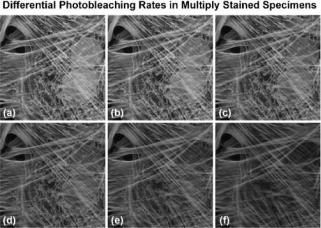
consideration when designing and executing fluorescence investigations. The two phenomena are distinct in that quenching is often reversible whereas photobleaching is not (154). Quenching arises from a variety of competing processes that induce nonradiative relaxation (without photon emission) of excited-state electrons to the ground state, which may be either intramolecular or intermolecular in nature. Because nonradiative transition pathways compete with the fluorescence relaxation, they usually dramatically lower or, in some cases, completely eliminate emission. Most quenching processes act to reduce the excited state lifetime and the quantum yield of the affected fluorophore.

A common example of quenching is observed with the collision of an excited state fluorophore and another (nonfluorescent) molecule in solution, resulting in deactivation of the fluorophore and return to the ground state. In most cases, neither of the molecules is chemically altered in the collisional quenching process. A wide variety of simple elements and compounds behave as collisional quenching agents, including oxygen, halogens, amines, and many elec- tron-deficient organic molecules (154). Collisional quenching can reveal the presence of localized quencher molecules or moieties, which via diffusion or conformational change, may collide with the fluorophore during the excited state lifetime. The mechanisms for collisional quenching include electron transfer, spin–orbit coupling, and intersystem crossing to the excited triplet state (154,155). Other terms that are often utilized interchangeably with collisional quenching are internal conversion and dynamic quenching.

A second type of quenching mechanism, termed static or complex quenching, arises from nonfluorescent complexes formed between the quencher and fluorophore that serve to limit absorption by reducing the population of active, excitable molecules (154,156). This effect occurs when the fluorescent species forms a reversible complex with the quencher molecule in the ground state, and does not rely on diffusion or molecular collisions. In static quenching, fluorescence emission is reduced without altering the excited state lifetime. A fluorophore in the excited state can also be quenched by a dipolar resonance energy transfer mechanism when in close proximity with an acceptor molecule to which the excited-state energy can be transferred nonradiatively. In some cases, quenching can occur through non molecular mechanisms, such as attenuation of incident light by an absorbing species (including the chromophore itself).

In contrast to quenching, photobleaching (also termed fading) occurs when a fluorophore permanently loses the ability to fluoresce due to photon-induced chemical damage and covalent modification (153–156). Upon transition from an excited singlet state to the excited triplet state, fluorophores may interact with another molecule to produce irreversible covalent modifications. The triplet state is relatively long lived with respect to the singlet state, thus allowing excited molecules a much longer timeframe to undergo chemical reactions with components in the environment (155). The average number of excitation and emission cycles that occur for a particular fluorophore before photobleaching is dependent on the molecular structure and the local environment (154,156).

Some fluorophores bleach quickly after emitting only a few photons, while others that are more robust can undergo thousands or even millions of cycles before bleaching.

Figure 17 presents a typical example of photobleaching (fading) observed in a series of digital images captured at different time points for a multiply stained culture of normal Tahr ovary (HJ1.Ov line) fibroblast cells. The nuclei were stained with DAPI (blue fluorescence), while the mitochondria and actin cytoskeleton were stained with MitoTracker Red CMXRos (red fluorescence) and an Alexa Fluor phalloidin derivative (Alexa Fluor 488; green fluorescence), respectively. Time points were taken in 2 min intervals using a fluorescence filter combination with bandwidths tuned to excite the three fluorophores simultaneously while also recording the combined emission signals. Note that all three fluorophores have a relatively high intensity in Fig. 17a, but the DAPI (blue) intensity starts to drop rapidly at two min and is almost completely gone at six min (Fig. 17f). The mitochondrial and actin stains are more resistant to photobleaching, but the intensity of both drops dramatically over the course of the timed sequence (10 min).

An important class of photobleaching events is represented by events that are photodynamic, meaning they involve the interaction of the fluorophore with a combination of light and oxygen (157–161). Reactions between fluorophores and molecular oxygen permanently destroy fluorescence and yield a free-radical singlet oxygen species that can chemically modify other molecules in living cells. The amount of photobleaching due to photodynamic events is a function of the molecular oxygen concentration and the proximal distance between the fluorophore, oxygen molecules, and other cellular components. Photobleaching can be reduced by limiting the exposure time of

Figure 17. Photobleaching in multiply stained specimens. Normal Tahr ovary fibroblast cells were stained with MitoTracker Red CMXRos (mitochondria; red fluorescence), Alexa Fluor 488 conjugated to phalloidin (actin; green fluorescence), and subsequently counterstained with DAPI (nuclei; blue fluorescence). Time points were taken in two-minute intervals over a 10 min period using a fluorescence filter combination with bandwidths tuned to excite the three fluorophores simultaneously while also recording the combined emission signals. (a–f) Time ¼0, 2, 4, 6, 8, 10 min, respectively.

474 MICROSCOPY, CONFOCAL

fluorophores to illumination or by lowering the excitation energy. However, these techniques also reduce the measurable fluorescence signal. In many cases, solutions of fluorophores or cell suspensions can be deoxygenated, but this is not feasible for living cells and tissues. Perhaps the best protection against photobleaching is to limit exposure of the fluorochrome to intense illumination (using neutral density filters) coupled with the judicious use of commercially available antifade reagents that can be added to the mounting solution or cell culture medium (153).

Under certain circumstances, the photobleaching effect can also be utilized to obtain specific information that would not otherwise be available. For example, in FRAP experiments, fluorophores within a target region are intentionally bleached with excessive levels of irradiation (82). As new fluorophore molecules diffuse into the bleached region of the specimen (recovery), the fluorescence emission intensity is monitored to determine the lateral diffusion rates of the target fluorophore. In this manner, the translational mobility of fluorescently labeled molecules can be ascertained within a very small (2–5 mm) region of a single cell or section of living tissue.

Although the subset of fluorophores that are advantageous in confocal microscopy is rapidly growing, many of the traditional probes that have been useful for years in widefield applications are still of little utility when constrained by fixed-wavelength laser spectral lines. Many of the limitations surrounding the use of fluorophores excited in the ultraviolet region will be eliminated with the introduction of advanced objectives designed to reduce aberration coupled to the gradual introduction of low cost, high power diode laser systems with spectral lines in these shorter wavelengths. The 405 nm blue diode laser is a rather cheap alternative to more expensive ion and Noble gas based ultraviolet lasers, and is rapidly becoming available for most confocal microscope systems. Helium– neon lasers with spectral lines in the yellow and orange region have rendered some fluorophores useful that were previously limited to widefield applications. In addition, new diode-pumped solid-state lasers are being introduced with emission wavelengths in the UV, violet, and blue regions.

Continued advances in fluorophore design, dual-laser scanning, multispectral imaging, endoscopic instruments, and spinning disk applications will also be important in the coming years. The persistent problem of emission crossover due to spectral overlap, which occurs with many synthetic probes and fluorescent proteins in multicolor investigations, benefits significantly from spectral analysis and deconvolution of lambda stacks. Combined, these advances and will dramatically improve the collection and analysis of data obtained from complex fluorescence experiments in live-cell imaging.

BIBLIOGRAPHY

1.Pawley JB, editor. Handbook of Biological Confocal Microscopy. New York: Plenum Press; 1995.

2.Paddock SW, editor. Confocal Microscopy: Methods and Protocols. Totowa (NJ): Humana Press; 1999.

3.Diaspro A, editor. Confocal and Two-Photon Microscopy: Foundations, Applications, and Advances. New York:

Wiley-Liss; 2002.

4.Matsumoto B, editor. Cell Biological Applications of Confocal Microscopy. Methods in Cell Biology, Vol. 70. New York:

Academic Press; 2002.

5.Sheppard CJR, Shotton DM. Confocal Laser Scanning Microscopy. Oxford (UK): BIOS Scientific Publishers; 1997.

6.Mu¨ ller M. Introduction to Confocal Fluorescence Microscopy. Maastricht, The Netherlands: Shaker; 2002.

7.Hibbs AR. Confocal Microscopy for Biologists. New York: Kluwer Academic; 2004.

8.Conn PM. Confocal Microscopy. Methods in Enzymology, Vol.

307.New York: Academic Press; 1999.

9.Corle TR, Kino GS. Confocal Scanning Optical Microscopy and Related Imaging Systems. New York: Academic Press; 1996.

10.Wilson T, editor. Confocal Microscopy. New York: Academic Press; 1990.

11.Gu M. Principles of Three-Dimensional Imaging in Confocal Microscopes. New Jersey: World Scientific; 1996.

12.Masters BR, editor. Selected Papers on Confocal Microscopy. SPIE Milestone Series, Vol. MS 131. Bellingham (WA): SPIE Optical Engineering Press; 1996.

13.Mason WT. Fluorescent and Luminescent Probes for Biological Activity. New York: Academic Press; 1999.

14.Peterman EJG, Sosa H, Moerner WE. Single-Molecule Fluorescence Spectroscopy and Microscopy of Biomolecular Motors. Ann Rev Phys Chem 2004;55:79–96.

15.Goldman RD, Spector DL. Live Cell Imaging: A Laboratory Manual. New York: Cold Spring Harbor Press; 2005.

16.Minsky M. Microscopy Apparatus. US Patent 3,013,467. 1961.

17.Minsky M. Memoir on Inventing the Confocal Scanning Microscopy. Scanning 1988;10:128–138.

18.Egger MD, Petran M. New Reflected-Light Microscope for Viewing Unstained Brain and Ganglion Cells. Science 1967;157:305–307.

19.Davidovits P, Egger MD. Photomicrography of Corneal Endothelial Cells in vivo. Nature (London) 1973;244:366–

20.Amos WB, White JG. How the Confocal Laser Scanning Microscope entered Biological Research. Biol Cell 2003;95:335–342.

21.Brakenhoff GJ, Blom P, Barends P. Confocal Scanning Light Microscopy with High Aperture Immersion Lenses. J Micros 1979;117:219–232.

22.Sheppard CJR, Wilson T. Effect of Spherical Aberration on the Imaging Properties of Scanning Optical Microscopes. Appl Opt 1979;18:1058.

23.Hamilton DK, Wilson T. Scanning Optical Microscopy by Objective Lens Scanning. J Phys E: Sci Instr 1986;19:52–54.

24.Spring KR, Inoue´ S. Video Microscopy: The Fundamentals. New York: Plenum Press; 1997.

25.Wilson T. Optical Sectioning in Confocal Fluorescence Microscopes. J Micros 1989;154:143–156.

26.Lichtmann JW. Confocal Microscopy. Sci Am Aug. 1994; 40–45.

27.White JG, Amos WB, Fordham M. An Evaluation of Confocal versus Conventional Imaging of Biological Structures by Fluorescence Light Microscopy. J Cell Biol 1987;105:41–48.

28.Swedlow JR, et al. Measuring Tubulin Content in Toxoplasma gondii: A Comparison of Laser-Scanning Confocal and Wide-Field Fluorescence Microscopy. Proc Natl Acad Sci USA 2002;99:2014–2019.

29.Stelzer EHK. Practical Limits to Resolution in Fluorescence Light Microscopy. In: Yuste R, Lanni F, Konnerth A, editors. Imaging Neurons: A Laboratory Manual. New York: Cold Spring Harbor Press; 2000. pp 12.1–12.9.

30.Rost FWD. Fluorescence Microscopy. Vol. 1. New York: Cambridge University Press; 1992.

31.Murray J. Confocal Microscopy, Deconvolution, and Structured Illumination Methods. In: Goldman RD, Spector DL, editors. Live Cell Imaging: A Laboratory Manual. New York: Cold Spring Harbor Press; 2005. pp 239–280.

32.Dickinson ME, et al. Multi-Spectral Imaging and Linear Unmixing Add a Whole New Dimension to Laser Scanning Fluorescence Microscopy. Biotechniques 2001;31:1272–1278.

33.Zimmermann T, Rietdorf J, Pepperkok R. Spectral Imaging and its Applications in Live Cell Microscopy. FEBS Lett 2003;546:87–92.

34.Lansford R, Bearman G, Fraser SE. Resolution of Multiple Green Fluorescent Protein Variants and Dyes using TwoPhoton Microscopy and Imaging Spectroscopy. J Biomed Opt 2001;6:311–318.

35.Hiraoka Y, Shimi T, Haraguchi T. Multispectral Imaging Fluorescence Microscopy for Living Cells. Cell Struct Funct 2002;27:367–374.

36.Gu Y, Di WL, Kelsell DP, Zicha D. Quantitative Fluorescence Energy Transfer (FRET) Measurement with Acceptor Photobleaching and Spectral Unmixing. J Microsc 2004;215:162– 173.

37.Ford BK, et al. Computed Tomography-Based Spectral Imaging for Fluorescence Microscopy. Biophys J 2001;80:986– 993.

38.Bach H, Renn A, Wild UP. Spectral Imaging of Single Molecules. Single Mol 2000;1:73–77.

39.Wilson T, Carlini AR. Three-Dimensional Imaging in Confocal Imaging Systems with Finite Sized Detectors. J Microsc 1988;149:51–66.

40.Murphy DB. Fundamentals of Light Microscopy and Electronic Imaging. New York: Wiley-Liss; 2001.

41.Wright SJ, Wright DJ. Introduction to Confocal Microscopy. In: Matsumoto B, editor. Cell Biological Applications of Confocal Microscopy. Methods in Cell Biology, Vol. 70. New York: Academic Press; 2002. pp 1–85.

42.Webb RH. Confocal Optical Microscopy. Rep Prog Phys 1996;59:427–471.

43.Wilhelm S, Gro¨bler B, Gluch M, Hartmut H. Confocal Laser Scanning Microscopy: Optical Image Formation and Electronic Signal Processing. Jena, Germany: Carl Zeiss Advanced Imaging Microscopy; 2003.

44.Ichihara A, et al. High-Speed Confocal Fluorescence Microscopy using a Nipkow Scanner with Microlenses for 3-D Imaging of Fluorescent Molecules in Real-Time. Bioimages 1996;4:57–62.

45.Inoue´ S, Inoue´ T. Direct-View High-Speed Confocal Scan- ner—The CSU-10. In: Matsumoto B, editor. Cell Biological Applications of Confocal Microscopy. Methods in Cell Biology, Vol. 70. New York: Academic Press; 2002. p 88–128.

46.Nakano A. Spinning-Disk Confocal Microscopy —A CuttingEdge Tool for Imaging of Membrane Traffic. Cell Struct Funct 2002;27:349–355.

47.Chong FK, et al. Optimization of Spinning Disk Confocal Microscopy: Synchronization with the Ultra-Sensitive EMCCD. In: Conchello JA, Cogswell CJ, Wilson T, editors. Three-Dimensional and Multidimensional Microscopy: Image Acquisition and Processing XI. Proc. SPIE. 2004; 5324: 65–76.

48.Sandison D, Webb W. Background Rejection and Signal-to- Noise Optimization in the Confocal and Alternative Fluorescence Microscopes. Appl Op 1994;33:603–610.

49.Centonze VE, White JG. Multiphoton Excitation Provides Optical Sections from Deeper within Scattering Specimens than Confocal Imaging. Biophys J 1998;75:2015.

50.Boccacci P, Bertero M. Image-Restoration Methods: Basics and Algorithms. In: Diaspro A, editor. Confocal and TwoPhoton Microscopy: Foundations, Applications, and Advances. New York: Wiley-Liss; 2002. pp 253–269.

51.Verveer PJ, Gemkow MJ, Jovin TM. A Comparison of Image Restoration Approaches Applied to Three-Dimensional Confocal and Wide-Field Fluorescence Microscopy. J Micros 1998;193:50–61.

52.Conchello JA, Hansen EW. Enhanced 3-D Reconstruction from Confocal Scanning Microscope Images. 1: Deterministic and Maximum Likelihood Reconstructions. Appl Op 1990;29: 3795–3804.

53.Al-Kofahi O, et al. Algorithms for Accurate 3D Registration of Neuronal Images Acquired by Confocal Scanning Laser Microscopy. J Micros 2003;211:8–18.

54.Conchello JA, et al., editors. Three-Dimensional and Multidimensional Microscopy: Image Acquisition and Processing. Vol. I–XII, Bellingham (WA): SPIE International Society for Optical Engineering; 1994–2005.

55.Centonze V, Pawley J. Tutorial on Practical Confocal Microscopy and use of the Confocal Test Specimen. In: Pawley JB, editor. Handbook of Biological Confocal Microscopy. New York: Plenum Press; 1995. p 549–570.

56.Gratton E, vandeVen MJ. Laser Sources for Confocal Microscopy. In: Pawley JB, editor. Handbook of Biological Confocal Microscopy. New York: Plenum Press; 1995. p 69–98.

57.Ashkin A, Dziedzic JM, Yamane T. Optical Trapping and Manipulation of Single Cells using Infrared Laser Beams. London 1987;330:769–771.

58.DeMaggio S. Running and Setting Up a Confocal Microscope Core Facility. In: Matsumoto B, editor. Cell Biological Applications of Confocal Microscopy. Methods in Cell Biology, Vol. 70. New York: Academic Press; 2002. p 475–486.

59.Spring KR. Detectors for Fluorescence Microscopy. In: Periasamy A, editor. Methods in Cellular Imaging. New York: Oxford University Press; 2001. p 40–52.

60.Art J. Photon Detectors for Confocal Microscopy. In: Pawley JB, editor. Handbook of Biological Confocal Microscopy. New York: Plenum Press; 1995. p 183–196.

61.Amos WB. Instruments for Fluorescence Imaging. In: Allan VJ, editor. Protein Localization by Fluorescence Microscopy: A Practical Approach. New York: Oxford University Press; 2000. pp 67–108.

62.Hergert E. Detectors: Guideposts on the Road to Selection. Photonics Design and Applications Handbook. 2001. pp H110–H113.

63.Piston DW, Patterson GH, Knobel SM. Quantitative Imaging of the Green Fluorescent Protein (GFP). In: Sullivan KF, Kay SA, editors. Green Fluorescent Proteins, Methods in Cell Biology, Vol. 58. New York: Academic Press; 1999. pp 31–47.

64.Carter DR. Photomultiplier Handbook: Theory, Design, Application. Lancaster (PA): Burle Industries, Inc.; 1980.

65.Cody SH, et al. A Simple Method Allowing DIC Imaging in Conjunction with Confocal Microscopy. J Microsc 2005;217: 265–274.

66.Chang IC. Acousto-Optic Devices and Applications. In: Bass M, Van Stryland EW, Williams DR, Wolfe WL, editors. Optics II: Fundamentals, Techniques, and Design. New York: McGraw-Hill; 1995. pp 12.1–12.54.

67.Wachman ES. Acousto-Optic Tunable Filters for Microscopy. In: Yuste R, Lanni F, Konnerth A, editors. Imaging Neurons: A Laboratory Manual. New York: Cold Spring Harbor Press; 2000. p 4.1–4.8.

68.Shonat RD, et al. Near-Simultaneous Hemoglobin Saturation and Oxygen Tension Maps in Mouse Brain using an AOTF Microscope. Biophy J 1997;73:1223–1231.

69.Wachman ES, Niu W, Farkas DL. Imaging Acousto-Optic Tunable Filter with 0.35-Micrometer Spatial Resolution. App Opt 1996;35:5220–5226.

70.Wachman ES. AOTF Microscope for Imaging with Increased Speed and Spectral Versatility. Biophys J 1997;73:1215–1222.

476MICROSCOPY, CONFOCAL

71.Chen Y, Mills JD, Periasamy A. Protein Localization in Living Cells and tissues using FRET and FLIM. Differentiation 2003;71:528–541.

72.Wallrabe H, Periasamy A. Imaging Protein Molecules using FRET and FLIM Microscopy. Curr Opin Biotech 2005;16: 19–27.

73.Day RN, Periasamy A, Schaufele F. Fluorescence Resonance Energy Transfer Microscopy of Localized Protein Interactions in the Living Cell Nucleus. Methods 2001;25:4–18.

74.Patterson GH, Lippincott-Schwartz J. A Photoactivatable GFP for Selective Photolabeling of Proteins and Cells. Science 2002;297:1873–1877.

75.Verkhusha VV, Lukyanov KA. The Molecular Properties and Applications of Anthozoa Fluorescent Proteins and Chromoproteins. Nature Biotechnol 2004;22:289–296.

76.Ando R, et al. An Optical Marker Based on the UV-Induced Green-to-Red Photoconversion of a Fluorescent Protein. Proc Natl Acad Sci USA 2002;99:12651–12656.

77.Sharma D. The Use of an AOTF to Achieve High Quality Simultaneous Multiple Label Imaging. Bio-Rad Technical Notes. San Francisco: Bio-Rad, Note 4; 2001.

78.Miyawaki A, Sawano A, Kogure T. Lighting up Cells: Labeling Proteins with Fluorophores. Nature Cell Biol 2003;5:S1–S7.

79.Zhang J, Campbell RE, Ting AY, Tsien RY. Creating New Fluorescent Probes for Cell Biology. Nature Rev Mol Cell Bio 2002;3:906–918.

80.Lippincott-Schwartz J, Patterson G. Development and Use of Fluorescent Protein Markers in Living Cells. Science 2003;300:87–91.

81.Klonis N, et al. Fluorescence Photobleaching Analysis for the Study of Cellular Dynamics. Eur Biophys J 2002;31:36–51.

82.Lippincott-Schwartz J, Altan-Bonnet N, Patterson GH. Photobleaching and Photoactivation: Following Protein Dynamics in Living Cells. Nature Cell Biol 2003;5:S7–S14.

83.Phair RD, Misteli T. Kinetic Modelling Approaches to in vivo Imaging. Nature Rev Mol Cell Bio 2002;2:898–907.

84.Politz JC. Use of Caged Fluorophores to Track Macromolecular Movement in Living Cells. Trends Cell Biol 1999;9:284–287.

85.Born M, Wolf E. Principles of Optics. New York: Cambridge University Press; 1999.

86.Stelzer EHK. Contrast, Resolution, Pixelation, Dynamic range, and Signal-to-Noise Ratio: Fundamental Limits to Resolution in Fluorescence Light Microscopy. J Microsc 1997;189:15–24.

87.Pawley J. Fundamental Limits in Confocal Microscopy. In: Pawley JB, editor. Handbook of Biological Confocal Microscopy. New York: Plenum Press; 1995. p 19–37.

88.Webb RH, Dorey CK. The Pixelated Image. In: Pawley JB, editor. Handbook of Biological Confocal Microscopy. New York: Plenum Press; 1995. p 55–67.

89.Jonkman JEN, Stelzer EHK. Resolution and Contrast in Confocal and Two-Photon Microscopy. In: Diaspro A, editor. Confocal and Two-Photon Microscopy: Foundations, Applications, and Advances. New York: Wiley-Liss; 2002. p 101–125.

90.Haugland RP. The Handbook: A Guide to Fluorescent Probes and Labeling Technologies. Chicago: Invitrogen Molecular Probes; 2005.

91.Lemasters JJ, et al. Confocal Imaging of Ca2þ, pH, Electrical Potential and Membrane Permeability in Single Living Cells. Methods Enzymol 1999;302:341–358.

92.Johnson I. Fluorescent Probes for Living Cells. Histochem J 1998;30:123–140.

93.Kasten FH. Introduction to Fluorescent Probes: Properties, History, and Applications. In: Mason WT, editor. Fluorescent and Luminescent Probes for Biological Activity. New York: Academic Press; 1999. p 17–39.

94.Coons AH, Creech HJ, Jones RN, Berliner E. Demonstration of Pneumococcal Antigen in Tissues by use of Fluorescent Antibody. J Immunol 1942;45:159–170.

95.Tsien RY. Building and Breeding Molecules to Spy on Cells and Tumors. FEBS Lett 2005;579:927–932.

96.Bruchez Jr M, et al. Semiconductor Nanocrystals as fluorescent Biological Labels. Science 1998;218:2013–2016.

97.Tsien RY, Waggoner A. Fluorophores for Confocal Microscopy. In: Pawley JB, editor. Handbook of Biological Confocal Microscopy. New York: Plenum Press; 1995. p 267–280.

98.Wessendorf MW, Brelje TC. Which Fluorophore is Brightest? A Comparison of the Staining Obtained Using Fluorescein, Tetramethylrhodamine, Lissamine Rhodamine, Texas Red and Cyanine 3.18. Histochemistry 1992;98:81–85.

99.Entwistle A, Noble M. The use of Lucifer Yellow, BODIPY, FITC, TRITC, RITC and Texas Red for Dual Immunofluorescence Visualized with a Confocal Scanning Laser Microscope. J Microsc 1992;168:219–238.

100.Darzynkiewicz Z. Differential Staining of DNA and RNA in Intact Cells and Isolated Cell Nuclei with Acridine Orange. Methods Cell Biol 1990;33:285–298.

101.Waring MJ. Complex Formation Between Ethidium Bromide and Nucleic Acids. J Mol Biol 1965;13:269–282.

102.Arndt-Jovin DJ, Jovin TM. Fluorescence Labeling and Microscopy of DNA. Fluores Microsc Living Cells Culture Part B Methods Cell Biol 1989;30:417–448.

103.Kubista M, Akerman B, Norden B. Characterization of Interaction between DNA and 40,6-Diamidino-2-phenylindole by Optical Spectroscopy. Biochemistry 1987;26:4545–4553.

104.Loewe H, Urbanietz J. Basic Substituted 2,6-Bisbenzimida- zole Derivatives: A Novel Series of Substances with Chemotherapeutic Activity. Arzneim-Forsch 1974;24:1927–1933.

105.Arndt-Jovin DJ, Jovin TM. Analysis and Sorting of Living Cells According to Deoxyribonucleic Acid Content. J Histochem Cytochem 1977;25:585–589.

106.Durand RE, Olive PL. Cytotoxicity, Mutagenicity and DNA Damage by Hoechst 33342. J Histochem Cytochem 1982; 30:111–116.

107.Panchuk-Voloshina N, et al. Alexa Dyes, A Series of New Fluorescent Dyes that Yield Exceptionally bright, Photostable Conjugates. J Histochem Cytochem 1999;47:1179–1188.

108.Berlier JE, et al. Quantitative Comparison of Long-Wavelength Alexa Fluor Dyes to Cy Dyes: Fluorescence of the Dyes and theirConjugates.JHistochemCytochem2003;51:1699–1712.

109.Mujumdar RB, et al. Cyanine Dye Labeling Reagents: Sulfoindocyanine Succinimidyl Esters. Bioconjugate Chem 1993;4:105–111.

110.Ballou B, et al. Tumor Labeling in vivo using CyanineConjugated Monoclonal Antibodies. Cancer Immunol Immunother 1995;41:257–263.

111.Zorov DB, Kobrinsky E, Juhaszova M, Sollott SJ. Examining Intracellular Organelle Function Using Fluorescent Probes. Circul Res 2004;95:239–252.

112.Stephens DG, Pepperkok R. The Many Ways to Cross the Plasma Membrane. Proc Natl Acad Sci USA 2001;98:4295–4298.

113.Rudolf R, Mongillo M, Rizzuto R, Pozzan T. Looking Forward to Seeing Calcium. Nature Rev Mol Cell Biol 2003;4:579–586.

114.Martin H, Bell MG, Ellis-Davies GC, Barsotti RJ. Activation Kinetics of Skinned Cardiac Muscle by Laser Photolysis of Nitrophenyl-EGTA. Biophys J 2004;86:978–990.

115.White C, McGeown G. Imaging of Changes in Sarcoplasmic Reticulum [Ca2þ] using Oregon Green BAPTA 5N and Confocal Laser Scanning Microscopy. Cell Calcium 2002;31:151–159.

116.Helm PJ, Patwardhan A, Manders EM. A Study of the Precision of Confocal, Ratiometric, Fura-2-Based [Ca2þ] Measurements. Cell Calcium 1997;22:287–298.

117.Rijkers GT, Justement LB, Griffioen AW, Cambier JC. Improved Method for Measuring Intracellular Caþþ with Fluo-3. Cytometry 1990;11:923–927.

118.Schild D, Jung A, Schultens HA. Localization of Calcium Entry through Calcium Channels in Olfactory Receptor Neurons using a Laser Scanning Microscope and the Calcium Indicator Dyes Fluo-3 and Fura-Red. Cell Calcium 1994;15: 341–348.

119.Willoughby D, Thomas RC, Schwiening CJ. Comparison of Simultaneous pH Measurements made with 8-Hydroxypyr- ene-1,3,6-trisulphonic acid (HPTS) and pH-Sensitive Microelectrodes in Snail Neurons. Pflugers Arch 1998;436:615–622.

120.Ozkan P, Mutharasan R. A Rapid Method for Measuring Intracellular pH using BCECF-AM. Biochim Biophys Acta 2002;1572:143.

121.Cody SH, et al. Intracellular pH Mapping with SNARF-1 and Confocal Microscopy. I: A Quantitative Technique for Living Tissue and Isolated Cells. Micron 1993;24:573–580.

122.Dubbin PN, Cody SH, Williams DA. Intracellular pH Mapping with SNARF-1 and Confocal Microscopy. II: pH Gradients within Single Cultured Cells. Micron 1993;24:581–586.

123.Poot M, et al. Analysis of Mitochondrial Morphology and Function with Novel Fixable Fluorescent Stains. J Histochem Cytochem 1996;44:1363–1372.

124.Keij JF, Bell-Prince C, Steinkamp JA. Staining of Mitochondrial Membranes with 10-Nonyl Acridine Orange, MitoFluor Green, and MitoTracker Green is Affected by Mitochondrial Membrane Potential Altering Drugs. Cytometry 2000;39: 203–210.

125.Reers M. et al. Mitochondrial Membrane Potential Monitored by JC-1 Dye. Methods Enzymol 1995;260:406–417.

126.Price OT, Lau C, Zucker RM. Quantitative Fluorescence of 5- FU-Treated Fetal Rat Limbs using Confocal Laser Scanning Microscopy and LysoTracker Red. Cytometry 2003;53A:9–21.

127.Kumar RK, Chapple CC, Hunter N. Improved Double Immunofluorescence for Confocal Laser Scanning Microscopy. J Histochem Cytochem 1999;47:1213–1217.

128.Suzuki T, Fujikura K, Higashiyama T, Takata K. DNA Staining for Fluorescence and Laser Confocal Microscopy. J Histochem Cytochem 1997;45:49–53.

129.Haugland RP. Coupling of Monoclonal Antibodies with Fluorophores. In: Davis WC, editor. Monoclonal Anibody Protocols, Methods in Molecular Biology. Vol. 45. Totowa, (NJ): Humana Press; 1995. p 205–221.

130.Pagano RE, Martin OC. Use of Fluorescent Analogs of Ceramide to Study the Golgi Apparatus of Animal Cells. In: Celis JE, editor. Cell Biology: A Laboratory Handbook. Vol. 2, 1998. p 507–512.

131.Cole L, Davies D, Hyde GJ, Ashford AE. ER-Tracker Dye and BODIPY-Brefeldin A Differentiate the Endoplasmic Reticulum and Golgi Bodies from the Tubular-Vacuole System in Living Hyphae of Pisolithus tinctorius. J Microsc 2000;197:239–249.

132.Jaiswal JK, Mattoussi H, Mauro JM, Simon SM. Long-Term Multiple Color Imaging of Live Cells using Quantum Dot Bioconjugates. Nature Biotechnol 2003;21:47–52.

133.Larson DR, et al. Water Soluble Quantum Dots for Multiphoton Fluorescence Imaging in vivo. Science 2003;300: 1434–1436.

134.Watson A, Wu X, Bruchez M. Lighting up Cells with Quantum Dots. Biotechniques 2003;34:296–303.

135.Michalet X, et al. Quantum Dots for Live Cells, in vivo Imaging, and Diagnostics. Science 2005;307:538–544.

136.Gao X, et al. In vivo Molecular and Cellular Imaging with Quantum Dots. Curr Opin Biotech 2005;16:63–72.

137.Lacoste TD, et al. Ultrahigh-Resolution Multicolor Colocalization of Single Fluorescent Probes. Proc Natl Acad Sci USA 2000;97:9461–9466.

138.Tsien RY. The Green Fluorescent Protein. Ann Rev Biochem 1998;67:509–544.

139.Sullivan KF, Kay SA, editors. Green Fluorescent Proteins, Methods in Cell Biology. Vol. 58. New York: Academic Press; 1999.

140.Conn PM, editor. Green Fluorescent Protein, Methods in Enzymology. Vol. 302. New York: Academic Press; 1999.

141.Hicks BW, editor. Green Fluorescent Protein, Methods in Molecular Biology. Vol. 183. Totowa (NJ): Humana Press; 2002.

142.Chalfie M, Kain S, editors. Green Fluorescent Protein: Properties, Applications, and Protocols. New York: Wiley-Liss; 1998.

143.Zimmer M. Green Fluorescent Protein: Applications, Structure, and Related Photophysical Behavior. Chem Rev 2002;102:759–781.

144.Chalfie M, et al. Green Fluorescent Protein as a Marker for Gene Expression. Science 1994;263:802–805.

145.Heim R, Cubitt AB, Tsien RY. Improved Green Fluorescence. Nature (London) 1995;373:664–665.

146.Heim R, Prasher DC, Tsien RY. Wavelength Mutations and Posttranslational Autoxidation of Green Fluorescent Protein. Proc Natl Acad Sci USA 1994;91:12501–12504.

147.Heim R, Tsien RY. Engineering Green Fluorescent Protein for Improved Brightness, Longer Wavelengths, and Fluorescence Resonance Energy Transfer. Curr Biol 1996;6: 178–182.

148.Wachter RM, et al. Structural Basis of Spectral Shifts in the Yellow-Emission Variants of Green Fluorescent Protein. Structure 1998;6:1267–1277.

149.Matz MV, et al. Fluorescent Proteins from Nonbioluminescent Anthozoa Species. Nature Biotechnol 1999;17:969–973.

150.Matz MV, Lukyanov KA, Lukyanov SA. Family of the Green Fluorescent Protein: Journey to the End of the Rainbow. BioEssays 2002;24:953–959.

151.Natural Animal Coloration can be Determined by a Nonfluorescent Green Fluorescent Protein Homolog. J Biol Chem 2000;275:25879–25882.

152.Song L, Hennink EJ, Young IT, Tanke HJ. Photobleaching Kinetics of Fluorescein in Quantitative Fluorescence Microscopy. Biophys J 1995;68:2588–2600.

153.Berrios M, Conlon KA, Colflesh DE. Antifading Agents for Confocal Fluorescence Microscopy. Methods Enzymol 1999; 307:55–79.

154.Lakowicz JR. Principles of Fluorescence Spectroscopy. New York: Kluwer Academic/Plenum Publishers; 1999.

155.Song L, Varma CA, Verhoeven JW, Tanke HJ. Influence of the Triplet Excited State on the Photobleaching Kinetics of Fluorescein in Microscopy. Biophys J 1996;70:2959–2968.

156.Herman B. Fluorescence Microscopy. New York: BIOS Scientific Publishers; 1998.

157.Bunting JR. A Test of the Singlet Oxygen Mechanism of Cationic Dye Photosensitization of Mitochondrial Damage. Photochem Photobiol 1992;55:81–87.

158.Byers GW, Gross S, Henrichs PM. Direct and Sensitized Photooxidation of Cyanine Dyes. Photochem Photobiol 1976; 23:37–43.

159.Dittrich PS, Schwille P. Photobleaching and Stabilization of Fluorophores used for Single Molecule Analysis with Oneand Two-Photon Excitation. Appl Phys B 2001;73:829–837.

160.Gandin E, Lion Y, Van de Vorst A. Quantum Yield of Singlet Oxygen Production by Xanthene Derivatives. Photochem Photobiol 1983;37:271–278.

161.Kanofsky JR, Sima PD. Structural and Environmental Requirements for Quenching of Singlet Oxygen by Cyanine Dyes. Photochem Photobiol 2000;71:361–368.

Further Reading

Willison JR. Signal Detection and Analysis, In: Bass, M. Van Stryland, E. W. Williams DR, Wolfe WL. Optics I: Fundamentals, Techniques, and Design. New York: McGraw-Hill; pp 1995. 18.1– 18.16.

See also CELLULAR IMAGING; FLUORESCENCE MEASUREMENTS;

ION-SENSITIVE FIELD EFFECT TRANSISTORS.