132 IMPEDANCE SPECTROSCOPY

17.Kubicek WG, et al. Development and evaluation of an impedance cardiac output system. Aerospace Med 1966;37:1208– 1212.

18.Nyboer J. Electrical impedance plethysmography: a physical and physiological aproach to peripheral vascular studies.

Circulation 1950;2:811–821.

¨

19. Yamamoto Y, Yamamoto T, Oberg PA. Impedance plethysmography in human limbs. Part 1: On electrodes and electrode geometry. Med Biol Eng Comput 1991;29:419–424.

¨

20. Yamamoto Y, Yamamoto T, Oberg PA. Impedance plethysmography in human limbs. Part 2: Influence of limb crosssectional areas. Med Biol Eng Comput 1992;30:518–524.

21. Lozano A, Rosell J, Pallas-Areny R. Errors in prolonged electrical impedance measurement due to electrode repositioning and postural changes. Physiol Meas 1995;16:121–130.

22. Risacher F, et al. Impedance plethysmography for the evaluation of pulse wave velocity in limbs. Med Biol Eng Comput 1992;31:318–322.

23. Hull R, et al. Impedance plethysmography: The relationship between venous filling and sensitivity and specificity for proximal vein thrombosis. Circulation 1978;58:898–902.

24. Brodie TG, Russel AE. On the determination of the rate of blood flow through an organ. J Physiol 1905;33:XLVII–XLVIII.

25. Seipel JH, Ziemnowicz SAR, O’Doherty DS. Cranial impedance plethysmography—rheoencephalography as a method for detection of cerebrovascular disease. In: Simonson E, McGavack TH, editors. Cerebral Ischemia. Springfield, IL: Charles C Thomas; 1965; p 162–179.

26. Hadjiev D. A new method for quantitative evaluation of cerebral blood flow by rheoencephalography. Brain Res 1968;8:213–215.

27. Netz J, Forner E, Haagemann S. Contactless impedance measurement by magnetic induction—a possible method for investigation of brain impedance. Physiol Meas 1993;14:463–471.

28. Geddes LA, Hoff HE, Hickman DM, Morre AG. The impedance pneumograph. Aerospace Med 1962;33:28–33.

29. Baker LE, Geddes LA, Hoff HE. Quantitative evaluation of impedance spirometry in man. Am J Med Elect 1965;4:73–77.

30. Nopp P, et al. Dielectric properties of lung tissue as a function of air content. Phys Med Biol 1993;38:699–716.

31. Brown BH, et al. Multifrequency imaging and modelling of respiratory related electrical impedance changes. Physiol Meas 1994;15(Suppl. A):1–12.

32. Nierman DM, et al. Transthoracic bioimpedance can measure extravascular water in acute lung injury. J Surg Res 1996;65:101–108.

33. Brack Th et al. Continuous and cooperation-independent monitoring of airway obstruction by a portable inductive plethysmograph. AJRCCM 2004;169:1.

34. Lo¨fgren B. The electrical impedance of a complex tissue and its relation to changes in volume and fluid distribution. Acta Physiol Scand 1951;23(Suppl. 81):1–51.

35. Schloerb PR, et al. Bioimpedance as a measure of total body water and body cell in surgical nutrition. Eur Surg Res 1986;18:1.

36. van Loan MD, et al. Association of bioelectric resistive impedance with fat-free mass and total body water estimates of body composition. Amer J Human Biol 1990;2:219–226.

37. Coulter WH. High speed automatic blood cell counter and cell size analyzer. Proc Nat Electron Conf 1956;12:1034.

38. Treo EF, et al. Comparative analysis of hematocrit measurements by dielectric and impedance techniques. IEEE Trans Biomed Eng 2005;MBE-52:549–552.

39. http://www.patentalert.com/docs/001/z00120411.shtml.

40. Yamakoshi KI, et al. Noninvasive measurement of hematocrit by electrical admittance plethysmography technique. IEEE Trans Biomed Eng 1989;27:156–161.

41.Mishra NN, et al. Bio-impedance sensing device (BISD) for detection of human CD4þ cells. Nanotech 2004, vol. 1, Proc 2004 NSTI Nanotechnology Conf 2004, p 228–231.

42.Brouillette RT, Morrow AS, Weese-Mayer DE, Hunt CE. Comparison of respiratory inductive plethysmography and thoracic impedance for apnea monitoring. J Ped 1987;111: 377–383.

43.Valta P, et al. Evaluation of respiratory inductive plethysmography in the measurement of breathing pattern and PEEPinduced changes in lung volume. Chest 1992;102:234–238.

44.Cohen KP, et al. Design of an inductive plethysmograph for ventilation measurement. Physiol Meas 1994;15:217–229.

45.Stro¨mberg TLT. Respiratory Inductive Plethysmography. Linko¨ping Studies in Science and Technologies Dissertations No. 417, 1996.

46.Malmivuo J, Plonsey R. Impedance plethysmography. In: Malmivuo J, Plonsey R, editors, Bioelectromagnetism. New York: Oxford University Press; 1995. Chapt. 25.

Further Reading

Foster KR, Schwan HP. Dielectric properties of tissue and biological materials. A critical review. Crit Rev Biomed Eng 1989;17:25–102.

Kaindl F, Polzer K, Schuhfried F. (1958, 1966, 1979): Rheographie. Darmstadt, Dr: Dietrich Steinkopff Verlag; 1958 (1st ed), 1966 (2nd ed), 1979 (3rd ed).

Morucci J-P, et al. Bioelectrical impedance techniques in medicine. Crit Rev Biomed Eng 1996;24:223–681.

Pethig R. Dielectric and Electronic Properties of Biological Materials. Chichester: Wiley; 1979.

Schwan HP. Determination of biological impedances. In: Nastuk WL, editor. Physical Techniques in Biological Research. Vol. VI (ptB) New York: Academic Press; 1963; p 323–407.

Schwan HP. Biomedical engineering: A 20th century interscience. Its early history and future promise. Med Biol Eng Comput 1999;37(Suppl. 2):3–13.

Stuchly MA, Stuchly SS. Dielectric properties of biological substances—tabulated. J Microw Power 1980;15:19–26.

Webster JG, editor. Medical Instrumentation—Application and Design. 3rd ed. New York: Wiley; 1998.

Gabriel C, Gabriel S. Compilation of the Dielectric Properties of Body Tissues at RF and Microwave Frequencies, 1996. Available at http://www.brooks.af.mil/AFRL/HED/hedr/reports/dielectric/ Report/Report.html.

See also BIOIMPEDANCE IN CARDIOVASCULAR MEDICINE; PERIPHERAL VASCULAR NONINVASIVE MEASUREMENTS.

IMPEDANCE SPECTROSCOPY

BIRGITTE FREIESLEBEN DE BLASIO

JOACHIM WEGENER

University of Oslo

Oslo, Norway

INTRODUCTION

Impedance spectroscopy (IS), also referred to as electrochemical impedance spectroscopy (EIS), is a versatile approach to investigate and characterize dielectric and conducting properties of materials or composite samples

(1). The technique is based on measuring the impedance

(i.e., the opposition to current flow) of a system that is being excised with weak alternating current or voltage. The impedance spectrum is obtained by scanning the sample impedance over a broad range of frequencies, typically covering several decades.

In the 1920, researchers began to investigate the impedance of tissues and biological fluids, and it was early known that different tissues exhibit distinct dielectric properties, and that the impedance undergoes changes during pathological conditions or after excision (2,3).

The advantage of IS is that it makes use of weak amplitude current or voltage that ensures damage-free examination and a minimum disturbance of the tissue. In addition, it allows both stationary and dynamic electrical properties of internal interfaces to be determined, without adversely affecting the biological system. The noninvasive nature of the method combined with its high information potential makes it a valuable tool for biomedical research and many medical applications are currently under investigation and development; this will be reviewed at the end of the article.

This article starts with providing a general introduction to the theoretical background of IS and the methodology connected to impedance measurement. Then, the focus will be on applications of IS, particularly devises for in vitro monitoring of cultured cell systems that have attracted widespread interest due to demand for noninvasive, mar- ker-free, and cost-effective methods.

THEORY

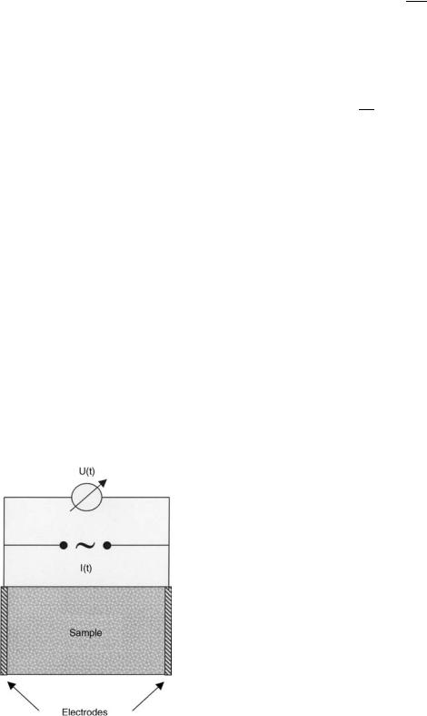
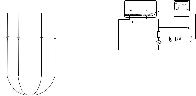
Impedance, Z, is a complex-valued vector that describes the ability of a conducting medium to resist flow of alternating current (ac). In a typical IS experiment (Fig. 1), a sinusoidal current I(t) signal with angular frequency v (v ¼ 2pf ) is passed through the sample and the resulting steady-state voltage U(t) from the excitation is

Figure 1. Schematic of a two-electrode setup to measure the frequency-dependent impedance of a sample that is sandwiched between two parallel plate electrodes.

measured. According to the ac equivalent of Ohm’s law, the impedance is given by the ratio of these two quantities

The impedance measurement is conducted with use of weak excitation signals, and in this case the voltage response will be sinusoid at the same frequency v as the applied current signal, but shifted in phase w. Introducing complex notation, Eq. 1 translates into

with U and I being the amplitudes of the voltage and

0 0 p

current, respectively, and i ¼ 1 being the imaginary unit. Thus, at each frequency of interest the impedance is described by two quantities: (1) its magnitude jZj, which is the ratio of the amplitudes of U(t) and I(t); and (2) the phase angle w between them. The impedance is measured over a range of frequencies between hertz and gigahertz, dependent on the type of sample and the problem to study.

The measured impedance can be divided into its real and imaginary components, that is, the impedance contribution arising from current in-phase with the voltage and 908 out-of-phase with the voltage

R ¼ ReðZÞ ¼ jZjcosðwÞ; X ¼ ImðZÞ ¼ jZjsinðwÞ (3)

The real part is called resistance, R, and the imaginary part is termed reactance, X. The reactive impedance is caused by presence of storage elements for electrical charges (e.g., capacitors in electrical circuit).

In some cases it is convenient to use the inverse quantities, which are termed admittance Y ¼ 1/Z, conductance G ¼ Re(Y), and susceptance B ¼ Im(Y), respectively. In the linear regime (i.e., when the measured signal is proportional to the amplitude of the excitation signal), these two representation are interchangeable and contain the same information. Thus, IS is also referred to as admittance spectroscopy.

INSTRUMENTATION

The basic devices for conducting impedance measurements consist of a sinusoid signal generator, electrodes, and a phase-sensitive amplifier to record the voltage or current. Commonly, a four-electrode configuration is used, with two current injecting electrodes and two voltage recording electrodes to eliminate the electrode–electrolyte interface impedance. As discussed below, some applications of IS make use of two-electrode arrangements in which the same electrodes are used to inject current and measure the voltage.

Since the impedance is measured by a steady-state voltage during current injection, some time is needed when changing the frequency before a new measurement can be performed. Therefore, it is very time consuming if each frequency has to be applied sequentially. Instead, it is common to use swept sine wave generators, or spectrum analyzers with transfer function capabilities and a white noise source. The white noise signal consists of the

134 IMPEDANCE SPECTROSCOPY

superposition of sine waves for each generated frequency, and the system is exposed to all frequencies at the same time. Fourier analysis is then used to extract the real and imaginary parts of the impedance.

The electrodes used for impedance experiments are made from biocompatible materials, such as noble metals, which in general is found not to have deleterious effect on biological tissue function. Electrode design is an important and complicated issue, which depends on several factors, including the spatial resolution required, the tissue depth, and so on. It falls beyond the scope of this article to go further into details. The interested readers are referred to the book by Grimnes and Martinsen (4) for a general discussion.

Common error sources in the measurements include impedance drift (e.g., caused by adsorption of particles on the electrodes or temperature variations). Ideally, the system being measured should be in steady-state throughout the time required to perform the measurement, but in practice this can be difficult to achieve. Another typical error source is caused by pick-up of electrical noise from the electronic equipment, and special attention must be paid to reduce the size of electric parasitics arising, for example, from cables and switches.

DATA PRESENTATION AND ANALYSIS

The most common way to analyze the experimental data is by fitting an equivalent circuit model to the impedance spectrum. The model is made by a collection of electrical elements (resistors, capacitors) that represents the electrical composition in the system under study.

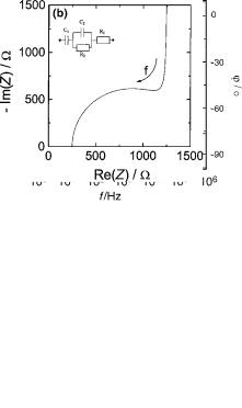
As a first step, it is useful to present the measured data by plotting log jZj and w versus log f in a so-called Bodediagram (Fig. 2a), and by plotting ImjZj versus RejZj named a Nyquist diagram or an impedance locus (Fig. 2b). The examples provided in Fig. 2 are made for an electrical circuit (insert Fig. 2b). While the first way of presenting the data shows the frequency-dependence explicitly, the phase angle w is displayed in the latter.

The impedance spectrum gives many insights to the electrical properties of the system, and with experience it is possible to make a qualified guess of a proper model based on the features in the diagrams (cf. Fig. 4). Similar to other spectroscopic approaches like infrared (IR) or ultraviolet (UV)/visible (vis), the individual components tend to show up in certain parts of the impedance spectrum. Thus, variations in the values of individual components alter the spectrum in confined frequency windows (Fig. 3).

For a given model, the total impedance (transfer function) is calculated from the individual components with use of Ohm’s and Kirchhoff’s laws. The best estimates for the parameters, that is, the unknown values of the resistors and capacitors in the circuit, are then computed with use of least-square algorithms. If the frequency response of the chosen model fits the data well, the parameter values are used to characterize the electrical properties of the system.

In order to fit accurately the equivalent circuit model impedance to the impedance of biomaterials, it is often necessary to include nonideal circuit elements, that is,

Figure 2. Different representations of impedance spectra. (a and b) visualize the frequency-dependent complex impedance of the electrical circuit shown in (b) with the network components:

R1 ¼ 250 V; R2 ¼ 1000 V; C1 ¼ 10 mF; C2 ¼ 1 mF. (a) Bodediagram presenting frequency-dependent impedance magnitude

jZj together with the phase shift w of the sample under investigation. (b) Wessel diagram locus of the same electrical network. The imaginary component of the impedance (reactance) is plotted against the real component (resistance). The arrow indicates the direction along which the frequency increases.

elements with frequency dependent properties. Such elements are not physically realizable with standard technical elements. Table 1 provides a list of common circuit elements that are used to describe biomaterials with respect to their impedance and phase shift. The constant phase element (CPE) portrays a nonideal capacitor, and was originally introduced to describe the interface impedance of noble metal electrodes immersed in electrolytic solutions

(5). The physical basis for the CPE in living tissue (and at electrode interfaces) is not clearly understood, and it is best treated as an empirical element. Another example is the Warburg impedance s that accounts for the diffusion limitation of electrochemical reactions (4).

It is important to place a word of caution concerning the equivalent circuit modeling approach. Different equivalent circuit models (deviating with respect to components or in the network structure) may produce equally good fits to the experimental data, although their interpretations are very different. It may be tempting to increase the number of elements in a model to get a better agreement between experiment and model. However, it may then occur that the model becomes redundant because the components cannot be quantified independently. Thus, an overly complex

model can provide artificially good fits to the impedance data, while at the same time highly inaccurate values for the parameters. Therefore, it is sound to use equivalent circuits with a minimum number of elements that can describe all aspects of the impedance spectrum (6).

Alternatively, the impedance data can be analyzed by deriving the current distribution in the system with use of differential equations and boundary values (e.g., the given excitation at the electrode surfaces). The parameters of the model impedances are then fitted to the data like described above. An example of this approach is be presented below, where it is used to analyze the IS of a cell-covered gold film electrode.

IMPEDANCE ANALYSIS OF TISSUE AND SUSPENDED CELLS

The early and pioneering work on bioimpedance is associated with the names of Phillipson, et al. (5). In these studies blood samples or pieces of tissue were examined in an experimental setup as shown in Fig. 1, and the dielectric properties of the biological system were investigated over a broad range of frequencies from hertz to gigahertz.

To understand the origin of bioimpedance, it is necessary to look at the composition of living material. Any tissue is composed of cells that are surrounded by an extracellular fluid. The extracellular medium contains proteins and polysaccharides that are suspended in an ionic solution and the electrical properties of this fluid

Figure 3. Calculated spectra of the impedance magnitude jZj for the electrical circuit shown in the insert of Fig. 2b when the network parameters have been varied individually. The solid line in each figure corresponds to the network parameters: R1 ¼ 250 V; R2 ¼ 1000 V; C1 ¼ 10 mF; C2 ¼ 1 mF. (a) Variation of C1: 10 mF (solid), 20 mF (dashed), 50 mF (dotted). (b) Variation of C2: 1 mF (solid), 0.5 mF (dashed), 0.1 mF (dotted). (c) Variation of R1: 1000 V (solid), 2000 V (dashed), 5000 V (dotted).

(d) Variation of R2: 250 V (solid), 500 V (dashed), 1000 V (dotted).

are determined by the mobility and concentration of the ions, primarily Naþ and Cl . The cell membrane marks the boundary between the interior and exterior environment, and consists of a 7–10 nm phospholipid bilayer. The membrane allows diffusion of water and small nonpolar molecules, while transport of ions and polar molecules requires the presence of integral transport proteins. On the inside, the cell contains a protein-rich fluid with specialized mem- brane-bound organelles, like the nucleus. For most purposes the fluid behaves as a pure ionic conductor. Thus, the cell membrane is basically a thin dielectric sandwiched between two conducting media and in a first approximation its impedance characteristics are mainly capacitive.

The simplest possible explanatory model for biological tissue (Fig. 4a-1) therefore consists of two membrane capa-

Table 1. Individual Impedance Contributions of Ideal and Empirical Equivalent Circuit Elements

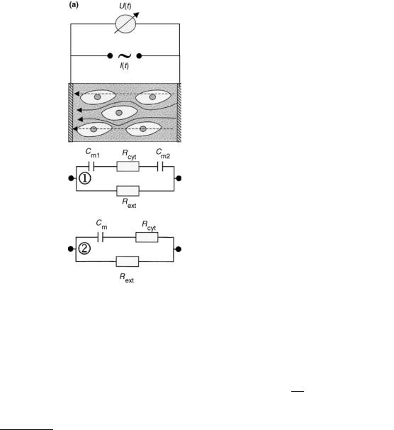
136 IMPEDANCE SPECTROSCOPY

Figure 4. (a) Schematics of the impedance measurement on living tissue. The arrows indicate the pathway of current flow for low frequencies (solid line) and high frequencies (dashed). Only at high frequencies the current flows through the cells. The electrical structure of tissue can be directly translated into equivalent circuit 1, which can be simplified to equivalent circuit 2. (b) Bodediagram for network 2 in Fig. 4a,

using Rext ¼ 1000 V; Rcyt ¼ 600 V; Cm ¼ 100 nF. (c) Impedance locus

generated with the same values.

citors Cm1 and Cm2 in series with a resistor of the cytosolic medium Rcyt, which in turn acts in parallel with the resistance of the conducting extracellular medium Rext. Since the two series capacitances of the membrane cannot be determined independently, they are combined to an overall capacitance Cm. The equivalent circuit model of this simple scenario (Fig. 4a-2) gives rise to a characteristic impedance spectrum, as shown with the Bode-diagram (Fig. 4b) and the Nyquist diagram (Fig. 4c). Impedance data for biological tissue is also often modeled by the socalled Cole–Cole equation (7)

This simple empirical model is identical to the circuit of Fig. 4, except that the capacitor is replaced by a CPE element. The impedance spectrum is characterized by four parameters ðDR; R1; a; tÞ, where R0; R1 is the lowand high frequency intercepts on the x axis in the Nyquist plot (cf. Fig. 4d), t is the time constant t ¼ DR C, and a is the CPE parameter. The impedance spectrum will be similar to Fig. 4b, c, but when a 6¼1, the semicircle in the Nyquist diagram is centered below the real axis, and the arc will appear flattened. For macroscopically heterogeneous biological tissue, the transfer function is written as a sum of Cole–Cole equations.

The features of the impedance spectrum Fig. 4b can be intuitively understood: at low frequencies the capacitor prevents current from flowing through Rcyt and the measured impedance arises from Rext. At high frequencies, with the capacitor having a very low impedance, the current is free to flow through both Rcyt, Rext. Thus, there is a

transition from constant-level impedance at low frequencies to another constant level. This phenomenon is termed dispersion, and will be discussed in the following.

A homogenous conducting material is characterized by a bulk property named the resistivity r0 having the dimensions of ohm centimeters (V cm). Based on this intrinsic parameter, the resistance may be defined by

where A is the cross-sectional area and L is the length of the material. Thus, by knowing the resistivity of the material and the dimensions of the system being studied, it is possible to estimate the resistance. Similarly, a homogeneous dielectric material is characterized by an intrinsic property called the relative permittivity e0, and the capacitance is defined by

where e0 is the permittivity of free space with dimension F/m, and A, d are the dimensions of the system as above. For most biological membranes, the area-specific capacitance is found to be quite similar, with a value of 1 mF cm 2 (8).

For historical reasons the notation of conductivity s0 with dimensions S m 1 and conductance (G ¼ s0A=d) has been preferred over resistance R and resistivity r, but the information content is the same, it is just expressed in a different way.

It is possible to recombine e0 and s0 by defining a complex permittivity e ¼ e0 þ e00, with ReðeÞ ¼ e0 and ImðeÞ ¼ e00. The

imaginary part accounts for nonideal capacitive behavior, for example, current within the dielectric due to bound charges giving rise to a viscous energy loss (dielectric loss). Therefore, e00 is proportional to s0, when adjusted for the conductivity that is due to migration s0 (9)

When a piece of biological material is placed between two electrodes, it is possible to measure the capacitance of the system and thereby to estimated the tissue permittivity e0. In general, e0 quantifies the ratio of the capacitance when a dielectric substance is placed between the electrodes, relative to the situation with vacuum in between. The increase of capacitance upon insertion of a dielectric material is due to polarization in the system in response to the electric field. For direct current (dc) or low frequency situations e0 is called the dielectric constant. When the frequency is increased, e0 often shows strong frequency dependence with a sigmoid character in a log–log plot of e0 versus frequency. This step-like decrease of the permittivity is referred to as a dielectric dispersion. The frequency fc at which the transition is half-complete is called the characteristic frequency, and is often expressed as time constant t with

Going back to Fig. 4c, the characteristic frequency is found directly as the point when the phase angle is at maximum.

The origin of dielectric dispersion in a homogeneous material is due to a phenomenon termed orientation polarization. Dipolar species within the material are free to move and orient themselves along the direction of the field, and therefore they contribute to the total polarization. However, when the frequency becomes too high, the dipoles can no longer follow the oscillation of the field, and their contribution vanishes. This relaxation causes the permittivity e0 to decrease.

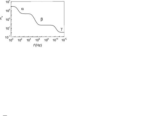
For heterogeneous samples like tissue additional relaxation phenomena occur, leading to more complex frequency dependence. In 1957, Schwan (10) defined three prominent dispersion regions of relevance for bioimpedance studies called a, b, and g, which is shown in Fig. 5. The dispersions are generally found in all tissue, although the time constant and the change in permittivity De0 between the different regions may differ (9).

Briefly stated, the a-dispersion originates from the cloud of counterions that are attracted by surface charges of the cell membrane. The counterions can be moved by an external electric field, thereby generating a dipole moment and relaxation. The b-dispersion, which is also called Maxwell–Wagner dispersion, is found in a window between kilohertz and megahertz (kHz and MHz). It arises due to the accumulation of charges at the interface between hydrophobic cell membranes and electrolytic solutions. Since the aqueous phase is a good conductor, whereas the membrane is not, mobile charges accumulate and charge up the membrane capacitor, thus, contributing to polarization. When the frequency gets too high, the charging is not complete, causing a loss of polarization. Finally,

Figure 5. Frequency-dependent permittivity e0 of tissue. The permittivity spectrum e0(f) is characterized by three major dispersions: a-, b-, and g-dispersion.

the g-dispersion is due to the orientation polarization of small molecules, predominantly water molecules.

Most IS measurements are performed at intermediate frequencies in the regime of the b-dispersion. In this frequency window, the passive electrical properties of tissue are well described with the simple circuit shown in Fig. 4 or by the Cole–Cole equation. The measurements can be used to extract information about extraand intercellular resistance, and membrane capacitance. For example, it has been shown that cells in liver tissue swell, when the blood supply ceases off (ischemia) and that the swelling of the cells can be monitored as an increase in the resistance of the extracellular space Rext (11). Cell swelling compresses the extracellular matrix around the cells, and thereby narrows the ion pathway in this region. Based on experiments like these, there is a good perspective and prognosis that IS may serve as a routine monitoring tool for tissue vitality even during the surgery.

APPLICATION: MONITORING OF ADHERENT CELLS

IN VITRO

The attachment and motility of anchorage dependent cell cultures is conveniently studied using a microelectrode setup. In this technique, cells are grown directly on a surface containing two planar metal electrodes, one microelectrode and one much larger counter electrode. The cells are cultured in normal tissue culture medium that serves as the electrolyte.

When current flows between the two electrodes, the current density, and the measured voltage drop, will be much higher at the small electrode. Therefore the impedance measurement will be dominated by the electrode polarization of the small electrode Zel. Instead, no significant polarization takes place at the larger counter electrode and its contribution to the measured impedance may be ignored. The electrode polarization impedance Zel acts physically in series with the resistance of the solution Rsol. Since the current density is high in a zone (the constrictional zone) proximal to the microelectrode, the electrolytic resistance will be dominated by the constriction resistance Rc in this region (Fig. 6). The total measured impedance may therefore be approximated by Z Zel þ Rc

(4). If necessary, Rc may be determined from high frequency measurements where the electrode resistance is

138 IMPEDANCE SPECTROSCOPY

Reference electrode

Z pol

Microelectrode

Figure 6. Schematic of two-electrode configuration.

infinitely small, that is, ReðZelÞ ! 0, and subtracted from the measured impedance to determine the impedance of the electrode–electrolyte interface.

When cells adhere on the small electrode, they constrain the current flow from the interface, increasing the measured impedance. The changes mainly reflects the capacitive nature of nonconducting lipid-bilayer membrane surrounding the cells. The cell membranes cause the current field to bend around the cells, much like if they were microscopic insulating particles. It is possible to follow both cell surface coverage and cell movements on the electrode, and morphological changes caused by physiological/pathological conditions and events may be detected. The technique may also be used to estimate cell membrane capacitances, and barrier resistance in epithelial cell sheets. In addition, the method is highly susceptible to vertical displacements of the cell body on the electrode with sensitivity in the nanometer range.

INSTRUMENTATION

The technique was introduced by Giaever and Keese in 1984 and referred to as Electrical Cell-Substrate Impedance Sensing (ECIS) (12,13). The ECIS electrode array consists of a microdisk electrode ð 5 10 4 cm2Þ and a reference electrode ð 0:15 cm2Þ; depending on the cell type to be studied, the recording disk electrode may contain a population of 20–200 cells. The electrodes are made from depositing gold film on a polycarbonate substrate over which an insulating layer of photoresist is deposited and delineated. A 1 V amplitude signal at fixed frequency (0.1– 100 kHz) is applied to the electrodes through a large resistor to create a controlled current of 1 mA, and the corresponding voltage across the cell-covered electrodes

Figure 7. The ECIS measurement setup.

is measured by a lock-in amplifier, which allows amplification of the relatively small signals. The amplifier is interfaced to a PC for data storage. The impedance is calculated from the measured voltage displayed in real time on the computer screen (Fig. 7). During the measurements the sample is placed in an incubator at physiological conditions.

The ECIS system is now commercially available, and the electrode slides allow multiple experiments to be performed at the same time (14). Some modifications to the technique have been described, such as a two-chamber sample well, which permit simultaneous monitoring on a set of empty electrodes being exposed to the same solution (15), platinized single-cell electrodes (15), and inclusion of a voltage divider technique to monitor the impedance across a range of frequencies (16). More recently, impedance studies have been performed using other types of electrode design. One approach has been to insert a perforated silicon-membrane between two platinium electrodes, there by allowing for two separate electrolytic solutions to exist on either side of the membrane (17). The results obtained with these techniques are generally identical to those obtained by the ECIS system.

MODEL OF ELECTRODE–CELL INTERFACE

To interpret ECIS-based impedance data, a model of the ECIS electrode–cell interface has been developed that allows determination of (1) the distance between the ventral cell surface and the substratum, (2) the barrier resistance, and (3) the cell membrane capacitance of confluent cell layers (18). The model treats the cells as disk shaped objects with a radius rc that are separated an average distance h from the substrate (Fig. 8). When cells cover the electrode, the main part of the current will flow through the thin layer of medium between the cell and the electrode, and leave the cell sheet in the narrow spacing between cells. However, the cell membrane, which is modeled as a capacitor (an insulating layer separating the conducting fluids of the solution and the cytosol) allows a parallel current flow to pass through the cells. The minor resistive component of the membrane impedance due to the presence of ionic channels is ignored in the calculations. By assuming that the electrode properties are not affected by the presence of cells, a boundary-value model of the current flow across the cell layer may be used to derive a relation

Cm

Rb

Ih

α

microelectrode

Figure 8. Model of current flow paths. The impedance changes associated with the presence of cells, arise in three different regions: from current flow under the cells quantified by a, from current flow in the narrow intercellular spacings causing the barrier resistance Rb. In parallel, some current will pass through the cell membranes giving rise to capacitive reactance Cm.

between the specific impedance of a cell-covered electrode Zcell and the empty electrode Zel

where I0; I1 are the modified Bessel functions of the first kind of order zero and one, Rb and r are the specific barrier resistance and resistivity of the solution, and Zm ¼2i=ðvCmÞ is the specific membrane impedance of the cells. A parameter a ¼ rcðr=hÞ0:5 is introduced as an assessment of the constraint of current flow under the cells. The impedance spectrum of an empty electrode and a cellcovered electrode is used to fit the three adjustable para-

meters ðRb; a; CmÞ.

The model outlined above has been further refined to describe polar epithelial cell sheets, treating separately the capacitance of the apical, basal, and lateral membranes (19). Some applications of the model will be discussed in the following sections.

MONITORING ATTACHMENT AND SPREADING

As a cell comes into contact with a solid surface, it forms focal contacts, primarily mediated by transmembrane proteins that anchor structural filaments in the cell interior to proteins on the substrate. During this process, the rounded cell spreads out and flattens on the surface, greatly increasing its surface area in contact with the electrode. The cell will also establish contacts with neighboring cells through particular cell–cell junctions, such as tight junctions, where strands of transmembrane proteins sew neighboring cells together, and gap junctions formed by clusters of intercellular channels, connecting the cytosol of adjacent cells.

The attachment process is normally studied using sin- gle-frequency measurements. Figure 9a and b show Bode

Figure 9. (a, b) Bode-diagrams of an ECIS electrode with confluent MDCK cells and an empty electrode. (c) Plot showing the division of the measured resistance of an ECIS electrode with confluent MDCK cells with the corresponding values of the empty electrode plotted versus log f.

plots for ECIS data of an empty electrode and an electrode with a confluent layer of epithelial MDCK cells. It is seen that the presence of cells primarily affects the impedance spectrum for intermediate frequencies between 1 and 100 kHz (Fig. 9a). At the highest frequencies, the two plots approach a horizontal plateau that represents the ohmic solution resistance between the working and the counter electrode. Within the relevant frequency window, the

140 IMPEDANCE SPECTROSCOPY

phase-shift plot for the data of the cell-covered electrode displays two extrema. At frequencies 200 Hz, the phase shift w is closest to zero, indicating that the contribution of the cells on the measured impedance is mainly resistive. At higher frequencies, the effect of the cell layer becomes more capacitive, and w starts approaching 908. The impedance spectrum of the empty electrode displays a single dispersion related to double-layer capacitance at the electrode interface.

The ideal measurement frequencies, where the presence of cells is most pronounced, are determined by dividing the impedance spectrum of a cell-covered electrode with the spectrum of a naked electrode. The same can be done for the resistance or capacitance spectrum, respectively. The most sensitive frequency for resistance measurements is typically found between 1 and 4 kHz (Fig. 9c), where the

ratio Rcell(f) / Rel(f) is at maximum. The capacitive contribution peaks at much larger frequencies, typically on the

order of 40 kHz, so that capacitance measurements are often performed at this higher frequency.

During the initial hours following the initial electrode– cell contact, the monitored impedance undergoes a characteristic steep increase. Once the spreading is complete, the impedance continues to fluctuate, reflecting the continuous morphological activities of living cells, for example, movements of cells on the electrode, either by local protrusions or directed movements of the entire cell body, or cell divisions (Fig. 10). The signal characteristics of the impedance during the spreading phase are generally found to be distinct for different cell cultures, both in terms of the duration of the initial gradient and its relative size in comparison to the impedance recorded from a the naked electrode (20). Also, characteristic impedance curves can be obtained by coating the electrode with different proteins (e.g., fibronectin, vitronectin) (21).

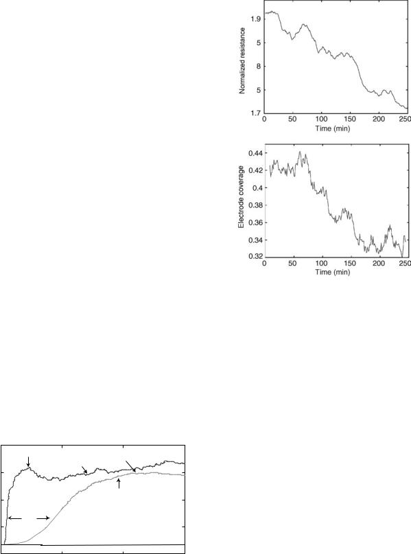
Simultaneous optical monitoring of a transparent ECIS electrode has allowed systematic comparison of cell confluence and measured impedance (22). Analysis of data from subconfluent MDCK epithelial cultures revealed a strong linear association between the two variables with cross-correlation coefficients > 0.9; the correlation was found to be equally strong in early and late cultures. This result indicates that 80% of the variance in the measured

Figure 10. Attachment assay of BSC and NRK fibroblastic cells followed for an interval of 15 h. The graph shows the measured resistance (4 kHz) as function of time; the spreading phase is indicated with arrows.

Figure 11. Correlation between resistance and cell coverage. The normalized resistance (4 kHz) versus time (upper panel), and the electrode coverage versus time (lower panel) during the same time interval. The measurement was started 32 h after the cells had been seeded out; the cross-correlation factor was r ¼ 0.94.

resistance (4 kHz) can be attributed to changes in cell coverage area (Fig. 11). Moreover, it was possible to link resistance variations to single-cell behavior during cell attachment, including cell-division (temporary impedance plateau) and membrane ruffling (impedance increase). The measured cell confluence was compared to the theoretical model (Eq. 9), neglecting the barrier resistance (i.e., Rb ¼ 0), and the calculated values were found to agree well with the data (Fig. 12). Studies like these might pave the way for standardized use of ECIS to quantify attachment and spreading of cell cultures.

IMPEDANCE SPECTROSCOPY AS A TRANDUCER IN CELL-BASED DRUG SCREENING

Another application of impedance spectroscopy with strong physiological and medical relevance is its use as transducer in ECIS-like experiments for cell-based drug screening assays. Here, the impedance readout can be used to monitor the response of cells upon exposure to a certain drug or a drug mixture. In these bioelectric hybrid assays the cells serve as the sensory elements and they determine the specificity of the screening assay while the electrodes are used as transducer to make the cell behavior observable. In the following example, endothelial cells isolated from bovine aorta (BAEC ¼ bovine aortic endothelial cells) were grown to confluence on gold-film electrodes since they

Figure 12. Theoretical prediction of cell coverage. Theoretical curve of normalized resistance plotted as function of cell coverage on the electrode. Normalized resistance and corresponding cell density are shown for four different registrations with circles. Time points indicate when the recordings were initiated with respect to the start of the culture; each circle corresponds to average values for 15 min time intervals.

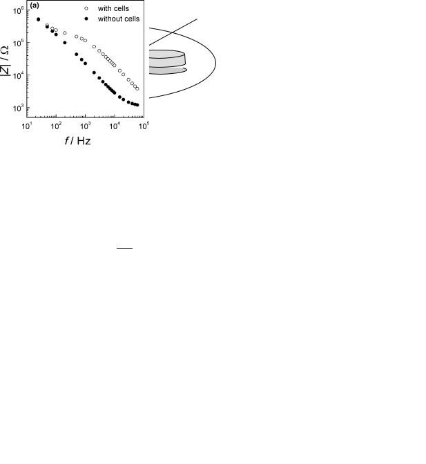
express cell-surface receptors (b-adrenoceptors) that are specific for adrenalin and derivatives (23,24). These b- adrenoceptors belong to the huge family of G-protein coupled receptors (GPCR) that are of great pharmaceutical relevance and impact. By measuring the electrical impedance of the cell-covered electrode, the stimulation of the cells by the synthetic adrenaline analogue isoprenaline (ISO) can be followed noninvasively in real time without any need to apply costly reagents or to sacrifice the culture (25). Experimentally, the most sensitive frequency for time-resolved impedance measurements is first determined from a complete impedance spectrum along an extended frequency range as depicted in Fig. 13. The figure compares the impedance spectrum of a circular gold-film electrode (d ¼ 2 mm) with and without a confluent monolayer of BAECs. The contribution of the cell layer to the total impedance of the system is most pronounced at frequencies close to 10 kHz, which is, thus, the most sensitive sampling frequency for this particular system. It is noteworthy that the most sensitive frequency may

Figure 13. Frequency-dependent impedance magnitude for a planar gold-film electrode (d ¼ 2 mm) with and without a confluent monolayer of BAEC directly growing on the electrode surface. The difference in impedance magnitude is maximum at a frequency of 10 kHz.

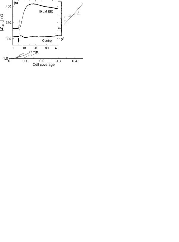
Figure 14. (a) Time course of the impedance magnitude at a sampling frequency of 10 kHz when a confluent monolayer of BAECs is exposed to 10 mM ISO or a corresponding vehicle control. (b) Dose-response relationship between the increase of impedance magnitude DZ and the concentration of isoproterenol applied. Quantitative analysis reveals an EC50 of 0.3 mM similar to the binding constant of ISO to b-adrenoceptors.

change with the electrode size and the individual electrical properties of the cells under study.

Figure 14a traces the time course of the impedance magnitude at a frequency of 10 kHz when confluent BAEC monolayers were either challenged with 10 mM ISO or a vehicle control solution at the time indicated by the arrow. The exchange of fluids produces a transient rise of the impedance by 10–20 V that is not caused by any cellular response, but mirrors the reduced fluid height within the measuring chamber. As expected, no response of the cells is seen in the control experiment. The cell population exposed to 10 mM of ISO shows a significant increase in electrical impedance that goes through a maximum 10 min after ISO application, and then slowly declines. The reason for the increase in impedance as observed after ISO stimulation is similar to what has been described for three-dimensional (3D) tissues above. The adrenaline derivative induces a relaxation of the cytoskeleton that in turn makes the cells flat out a bit more. As a consequence the extracellular space between adjacent cells narrows and increases the impedance of the cell layer. Note that the time resolution in these measurements is 1 s so that even much faster cell responses than the one studied here can be monitored in real time. Moreover, no labeled probe had to be applied and

142 IMPEDANCE SPECTROSCOPY

the sensing voltages used for the measurement (U0 ¼ 10 mV) are clearly noninvasive.

From varying the ISO concentration, a dose-response relationship (Fig. 14b) can be established which is similar to those derived from binding studies using radiolabeled ligands. Fitting a dose-response transfer function to the recorded data returns the concentration of half-maximum

efficiency EC50 as (0.3 0.1) mM, which is in close agreement to the binding constant of ISO to b-adrenoceptors on

the BAEC surface as determined from binding assays with radiolabeled analogs (23).

These kind of electrochemical impedance measurements are also used to screen for potent inhibitors of cell-surface receptors. Staying with the example discussed in the preceding paragraph, the blocking effect of Alprenolol (ALP), a competitive inhibitor of b-adrenoceptors (b-blocker), is demonstrated. Preincubation of BAEC with ALP blocks the stimulating activity of ISO, as shown in Fig. 15. The figure compares the time course of the impedance magnitude at a frequency of 10 kHz when BAEC monolayers were stimulated with 1 mM ISO either in absence of the b-blocker (a) or after preincubation (b).

Figure 15. (a) Time course of the impedance magnitude at a sampling frequency of 10 kHz, when confluent BAEC are exposed to 1 mM ISO. (b) Time course of the impedance magnitude of a confluent monolayer of BAECs upon sequential exposure to 10 mM of the b-blocker ALP and 1 mM ISO 20 min later. The b-adrenergic impedance increase is omitted by the b-blocker. Intactness of the signal transduction cascade is verified by addition of forskolin (FOR), a receptor independent activator of this signal transduction pathway.

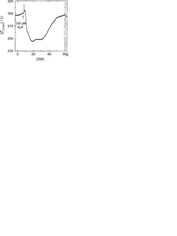
Figure 16. Time course of the impedance magnitude at a sampling frequency of 10 kHz when a confluent BAEC monolayer is exposed to an over dose of the b-blocker alprenolol (100 mM ALP). Addition of ALP is indicated by the arrow.

When the cell layers were incubated with 10 mM ALP prior to the addition of 1 mM ISO, the cells do not show any ISO response indicating that a 10-fold increase of ALP was sufficient to block activation of the receptors. To prove that the cells were not compromised in any way during these experiments the same signal transduction cascade was triggered via a receptor-independent way at the end of each experiment. This can be easily done by application of FOR, a membrane permeable drug that intracellularly activates the same enzyme that is triggered by ISO binding to the receptor. Forskolin stimulation of those cells that had been blocked with ALP earlier in the experiment induces a strong increase of electrical impedance indicating that the intracellular transduction pathways are functional (Fig. 15b).

Besides screening for the activity of drugs in cell-based assays, these kind of measurements are also used to check for unspecific side effects of the compounds of interest on cell physiology. Dosage of ALP and many of its fellow b- blockers has to be adjusted with great care since these lipophilic compounds are known to integrate nonspecifically into the plasma membrane. As shown in Fig. 15b, application of 10 mM ALP does not show any measurable side effects. Using ALP in concentrations of 100 mM induces a transient but very pronounced reduction of the electrical impedance (Fig. 16). This decrease in impedance may be the result of the interaction of ALP with the plasma membrane or an induced contraction of the cell bodies.

The preceding examples showed that impedance measurements of cell-covered gold electrodes in which the cells serve as sensory elements can be used in screening assays for pharmaceutical compounds, but also for cytotoxicity screening. The interested reader is referred to Ref. 26 and 27.

SUMMARY AND OUTLOOK

Impedance spectroscopy is a general technique with important applications in biomedical research and medical diagnostic practice. Many new applications are currently under investigation and development. The potential of the

technique is obviously great, since it is noninvasive, easily applied, and allows on-line monitoring, while requiring low cost instrumentation. However, there are also difficulties and obstacles related to the use of IS. Foremost, there is no separate access to the individual processes and components of the biological system, only the total impedance is measured, and this signal must be interpreted by some chosen model. There are many fundamental issues yet to be solved, both connected with understanding the origin of bioimpedance, methodological problems with finding standardized ways of comparing different samples, as well as technical issues connected with the equipment used to probe bioimpedance.

Prospective future in vivo applications include quantification of ischemia damage during cardiac surgery (28) and organ transplantation (29), as well as graft rejection monitoring (30). Impedance spectroscopy are also used for tissue characterization, and recently a device for breast cancer screening became commercially available. Multifrequency electrical impedance tomography (EIT) performing spatially resolved IS is a potential candidate for diagnostic imaging devices (31), but due to poor resolution power compared to conventional methods like MR, only few clinical applications are described.

The use of impedimetric biosensor techniques for in vitro monitoring of cell and tissue culture is promising. With these methods, high sensitivity measurements of cell reactions in response to various stimuli have been realized, and monitoring of physiological–pathological events is possible without use of marker substances. The potential applications cover pharmaceutical screening, monitoring of toxic agents, and functional monitoring of food additives. Microelectrode-based IS is interesting also for scientific reasons since it allows studying the interface between cells and technical transducers and supports the development of implants and new sensor devices (32).

Finally, affinity-based impedimetric biosensors represent an interesting and active research field (33) with many potential applications, for example, immunosensors monitoring impedance changes in response to antibody– antigen reactions taking place on electrode surfaces.

BIBLIOGRAPHY

1.Macdonald JR. Impedance Spectroscopy. New York: John Wiley & Sons; 1987.

2.Fricke H, Morse S. The electrical capacity of tumors of the breast. J Cancer Res 1926;10:340–376.

3.Schwan H. Mechanisms Responsible for Electrical Properties of Tissues and Cell Suspensions. Med Prog Technol 1993;19: 163–165.

4.Grimnes S, Martinsen ØG. Bioimpedance and Bioelectricity basics. Cornwall: Academic Press; 2000.

5.McAdams E, Lackermeier A, McLaughlin J, Macken D, Jossinet J. The linear and non-linear electrical properties of the electrode-electrolyte-interface. Biosens Bioelectron 1995;10: 67–74.

6.Kottra G, Fromter E. Rapid determination of intraepithelial resistance barriers by alternating current spectroscopy. II. Test of model circuits and quantification of results. Pflugers Arch 1984;402:421–432.

7.Cole K, Cole R. Dispersion and adsorption in dielectrics. I.. alternating current characteristics. J Chem Phys 1941;9: 341–351.

8.Cole Ks. Membrane, Ions and Impulses. Berkeley (CA): University of California Press; 1972.

9.Kell D. Biosensor. Fundamentals and Applications. Turner A, Karube I, Wilson G, editors. Oxford Science Publications; 1987. pp 427–468.

10.Schwan H. Electrical properties of tissue and cell suspensions. Advances in biological and medical physics. Lawrence J, Tobias C, editors. New York: Academic Press; 1957. pp 147– 209.

11.Gersing E. Impedance spectroscopy on living tissues for determination of the state of organs. Bioelectrochem Bioenenerg 1998;45:149.

12.Giaever I, Keese CR. Monitoring fibroblast behavior in tissue culture with an applied electric field. Proc Natl Acad Sci 1984;81:3761–3764.

13.Giaever I, Keese CR. A morphological biosensor for mammalian cells. Nature (London) 1993;366:591–592.

14.Applied Biophysics, Inc. 2002.

15.Connolly P, et al. Extracellular electrodes for monitoring cell cultures. IOP Publishing; 1989.

16.Wegener J, Sieber M, Galla HJ. Impedance analysis of epithelial and endothelial cell monolayers cultured on gold surfaces. J Biochem Biophys Methods 1996;76:327–330.

17.Hagedorn R, et al. Characterization of cell movement by impedance measurements on fibroblasts grown on perforated Si-membranes. Biochem Biophys Acta—Molecular Cell Res 1955;1269:221–232.

18.Giaever I, Keese C. Micromotion of mammalian cells measured electrically. Proc Natl Acad Sci USA 1991;88:7896– 7900.

19.Lo CM, Keese CR, Giaever I. Impedance analysis of MDCK cells measured by electric cell-substrate impedance sensing. Biophys J 1995;69:2800–2807.

20.Giaever I, Keese CR. Use of electric fields to monitor the dynamical aspect of cell behavior in tissue culture. IEEE Trans Biomed Eng 1986;33:242–247.

21.Mitra P, Keese CR, Giaever I. Electrical measurements can be used to monitor the attachment and spreading of cells in tissue culture. BioTechniques 1991;11:504–510.

22.De Blasio BF, Laane M, Walmann T, Giaever I. Combining optical and electrical impedance techniques for quantitative measurements of confluence in MDCK-I cell cultures. BioTechniques 2004;36:650–662.

23.Zink S, Roesen P, Sackmann B, Lemoine H. Regulation of endothelial permeability by beta-adrenoceptor agonists: Contribution of beta 1- and beta 2-adrenoceptors. Biochim Biophys Acta 1993;1178:286–298.

24.Zink S, Roesen P, Lemoine H. Microand macrovascular endothelial cells in beta-adrenergic regulation of transendothelial permeability. Am J Physiol 1995;269:C1209– C1218.

25.Wegener J, Zink S, Roesen P, Galla H. Use of electrochemical impedance measurements to monitor betaadrenergic stimulation of bovine aortic endothelial cells. Pflugers Arch 1999;437:925–934.

26.Arndt S, et al. Bioelectrical impedance assay to monitor changes in cell shape during apoptosis. Biosens Bioelectron 2004;19:583–594.

27.Keese C, Karra N, Dillon B, Goldberg A, Giaever I. Cellsubstratum interactions as a predictor of cytotoxity. In Vitro Mol Toxicol 1998;11:183–191.

28.Benvenuto, et al. Impedance microprobes for myocardial ischemia monitoring. 1st Annual International IEEE-EMBS. Lyon, France; 2000. p 234–238.