


The ABC’s of AutoLISP by George Omura
(setq cent (osnap cpt1 "center"))
Here the point picked previously as the point on the circle cpt1 is used in conjunction with the osnap function to obtain the center point of the circle. The syntax for osnap is:
(osnap [point value][osnap mode])
The osnap function acts in the same way as the osnap overrides. If you use the center osnap override and pick a point on the circle, you get the center of the circle. Likewise, the osnap function takes a point value and applies an osnap mode to it to obtain a point. In this case, osnap applies the center override to the point cpt1 which is located on the circle. This gives us the center of the circle which is assigned to the symbol cent.
The next expression obtains the circle's radius
(setq rad1 (distance cpt1 cent))
The distance function is used to get the distance from cpt1, the point located on the circle, to cent, the center of the circle. This value is assigned to the symbol rad1.
Finding Points Using Trigonometry
At this point, we have all the known points we can obtain without utilizing some math. ultimately, we want to find the intersection point between the circle and the cut axis. By using the basic trigonometric functions, we can derive the relationship between the sides of triangle. In particular, we want to look for triangles that contain right angles. If we analyze the known elements to our problem, we can see that two triangles can be used to find one intersection on the circle (See figure 6.14)
Figure 6.14: Triangles used to find the intersection
128
Copyright © 2001 George Omura,,World rights reserved

The ABC’s of AutoLISP by George Omura
In our analysis, we see that we can find a point along the cut axis that describes the corner of a right triangle. To find this point, we only need an angle and the length of the hypotenuse of the triangle. We can then apply one of the basic trigonometric functions shown in figure 6.15 to our problem.
Figure 6.15: Basic trigonometric functions
The sine function is the best match to information we have.
sine(angle) = opposite side / hypotenuse
This formula has to be modified using some basic algebra to suite our needs:
opposite side = hypotenuse * sine (angle)
Before we can use the sine function, we need to find the angle formed by points lpt1, lpt2 and cent (see figure 6.16).
Figure 6.16: Angle needed to before the sine function can be used.
129
Copyright © 2001 George Omura,,World rights reserved

The ABC’s of AutoLISP by George Omura
The following function does this for us:
(setq ang1 (- (angle lpt1 cent) (angle lpt1 lpt2)))
The first of these three functions finds the angle described by points lpt1 and lpt1. The second expression finds the angle from lpt1 to the center of the circle. The third line finds the difference between these two angles to give us the angle of the triangle we need (see figure 6.17).
Figure 6.17: The sine expression written to accommodate the known elements.
We also need the length of the hypotenuse of the triangle. this can be gotten by finding the distance between lpt1 and the center of the triangle:
(setq dst1 (distance lpt1 cent))
The length of the hypotenuse is saved as the variable dst1. We can now apply our angle and hypotenuse to the formula:
opposite side = hypotenuse * sine (angle) becomes
(setq dst2 (* dst1 (sin ang1)))
Now we have the length of the side of the triangle but we need to know the direction of that side in order to find the corner point of the triangle. We already know that the direction is at a right angle to the cut axis. therefore, we can determine the right angle to the cut axis by adding the cut axis angle to 1.57 radians (90 degrees)(see figure 6.18). The following expression does this for us:
(setq ang2 (- (angle lpt1 lpt2) 1.57))
130
Copyright © 2001 George Omura,,World rights reserved
The ABC’s of AutoLISP by George Omura
Figure 6.18: Finding the angle of the opposite side of the triangle.
We are now able to place the missing corner of the triangle using the polar function (see figure 6.19).
(setq wkpt (polar cent ang2 dst2))
Figure 6.19: Finding the workpoint wkpt.
131
Copyright © 2001 George Omura,,World rights reserved

The ABC’s of AutoLISP by George Omura
We assign the corner point location to the variable wkpt. We're still not finished with our little math exercise, however. We still need to find the intersection of the cut axis to the circle. Looking at our problem solving sketch, we can see that yet another triangle can be used to solve our problem. We know that the intersection lies along the cut axis. We can describe a triangle whose corner is defined by the intersection of the circle and the cut axis (see figure 6.20).
Figure 6.20: The triangle describing one intersection point.
We also already know two of the sides of this new triangle. One is the radius of the circle stored as the variable rad1. The other is the side of the triangle we used earlier stored as the variable dst2. The most direct way to find the intersection is to apply the Pythagorean Theorem shown in figure 6.21.
Figure 6.21: The Pythagorean Theorem
132
Copyright © 2001 George Omura,,World rights reserved
The ABC’s of AutoLISP by George Omura
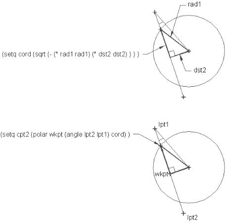
Again we must apply algebra to derive a formula to suite our needs. The formula:
c2 = a2 - b2
becomes the expression:
(setq cord (sqrt(-(* rad1 rad1)(* dst2 dst2))))
We assign the distance value gotten from the Pythagorean Theorem to the variable cord. Using the Polar function, we can now find one intersection point between the circle and the cut axis:
(setq cpt2 (polar wkpt (angle lpt2 lpt1) cord))
In this expression, we find one intersection by applying the angle described by lpt1 and lpt2 and the distance described by cord to the polar functions (see figure 6.22).
Figure 6.22: Finding the location of an intersection point.
133
Copyright © 2001 George Omura,,World rights reserved
The ABC’s of AutoLISP by George Omura
Since the two intersection points are symmetric about point wkpt, the second intersection point is found by reversing the direction of the angle in previous expression:
(setq cpt3 (polar wkpt (angle lpt1 lpt2) cord))
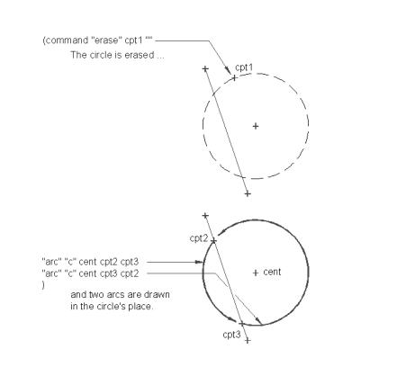
Finally, we can get AutoCAD to do the actual work of cutting the circle:
(command "erase" cpt1 "" "arc" "c" cent cpt2 cpt3 "arc" "c" cent cpt3 cpt2
)
)
Actually, we don't really cut the circle. Instead, the circle is erased entirely and replaced with two arcs (see figure 6.23).
Figure 6.23: Drawing the new circle.
134
Copyright © 2001 George Omura,,World rights reserved