The ABC’s of AutoLISP by George Omura

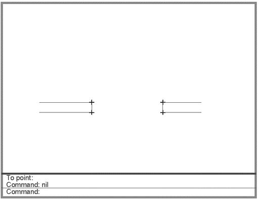
pick the upper line near its midpoint. The two line break and are joined at their break points to form an opening (see figure 6.4)

Figure 6.4: The lines after using Break2

Now draw several parallel lines at different orientations and try the Break2 program on each pair of lines. Break2 places an opening in a pair of parallel lines regardless of their orientation. Let's look at how break2 accomplishes this.

Understanding the Angle, Distance, and Polar Functions

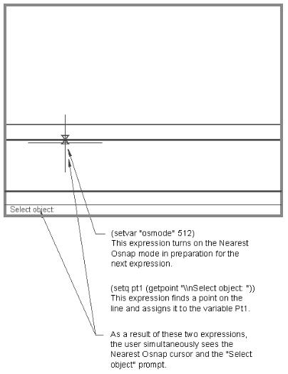
The first line after defun function uses the setvar function to set the osnap system variable to the nearest mode.

(defun C:BREAK2 (/ pt1 pt2 pt3 pt4 pt0 ang1 dst1)

116

Copyright © 2001 George Omura,,World rights reserved

The ABC’s of AutoLISP by George Omura

(setvar "osmode" 512)

This ensures that the point the user picks at the next prompt is exactly on the line. It also give the user a visual cue to pick something since the osnap cursor appears.

When setvar is used with the osmode system variable, a numeric code must also be supplied. This code determines the osnap mode to be used. Table 6.1 shows a list of the codes and their meaning.

Table 6.1: Osmode codes and their meaning

The next line prompts the user to select an object using the getpoint function:

(setq pt1 (getpoint "\nSelect object: "))

Here, the variable pt1 is used to store the first point location for the break. Since the nearest osnap mode is used, the osnap cursor appears and the point picked falls exactly on the line (see Figure 6.5).

117

Copyright © 2001 George Omura,,World rights reserved

The ABC’s of AutoLISP by George Omura

Figure 6.5: Getting a point using the "nearest" osnap mode.

Next, another prompt asks the user to pick another point:

(setq pt2 (getpoint pt1 "\nEnter second point: "))

The variable pt2 is assigned a point location for the other end of the break. The next line:

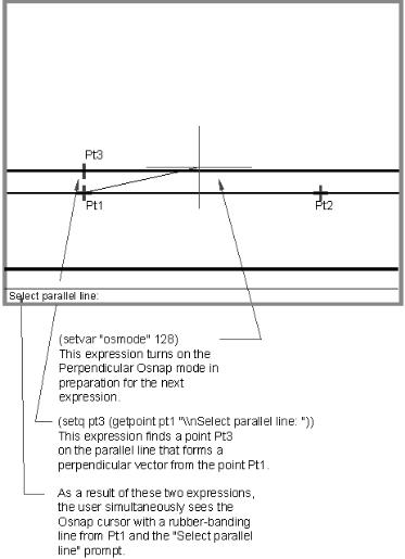
(setvar "osmode" 128)

sets the osnap mode to perpendicular in preparation for the next prompt:

(Setq pt3 (getpoint pt1 "\nSelect parallel line: "))

118

Copyright © 2001 George Omura,,World rights reserved

The ABC’s of AutoLISP by George Omura

Here, the user is asked to select the line parallel to the first line. The user can pick any point along the parallel line and the perpendicular osnap mode ensures that the point picked on the parallel line is "perpendicular" to the first point stored by the variable pt1. The perpendicular osnap mode will only work, however, if a point argument is supplied to the Getpoint function. In this case, the point pt1 is supplied as a reference from which the perpendicular location is to be found (see figure 6.6). This new point variable pt3 will be important in calculating the location of the two break points on the parallel line.

Figure 6.6: Picking the point perpendicular to the first point.

119

Copyright © 2001 George Omura,,World rights reserved

The ABC’s of AutoLISP by George Omura

The next line sets the osnap mode back to "none":

(Setvar "osmode" 0)

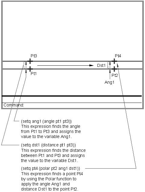
The next two lines find the angle and distance described by the two point variables pt1 and pt3.

(setq ang1 (angle pt1 pt3))

(setq dst1 (distance pt1 pt3))

You can obtain the angle described by two points using the Angle function. Angles syntax is:

( angle [coordinate list][coordinate list] )

The arguments to angle are always coordinate lists. The lists can either be variables or quoted lists.

Angle returns a value in radians. You looked at radians briefly in chapter 4. A radian is system to measure angles based on a circle of 1 unit radius. In such a circle, an angle can be described as a distance along the circle's circumference. You may recall from high school geometry that a circle's circumference is equal to 2 times pi times its radius. since the hypothetical circle has a radius of 1, we drop the one from the equation.

circumference = 2pi

90 degrees is equal to one quarter the circumference of the circle or pi/2 radians or 1.5708 (see figure 6.7). 180 degrees is equal to half the circumference of a circle or 1 pi radians or 3.14159. 360 degrees is equal the full circumference of the circle or to 2 pi radians or 6.28319.

A simple formula to convert degrees to radians is:

radians * 57.2958

To convert degrees to radians the formula is:

degrees * 0.0174533

Angle uses the current UCS orientation as its basis for determining angles. Though you can supply 3 dimensional point values to angle, the angle returned is based on a 2 dimensional projection of those points on the current UCS (see figure 6.7). Finally, radians are always measured with a counterclockwise directions being positive.

120

Copyright © 2001 George Omura,,World rights reserved

The ABC’s of AutoLISP by George Omura

Figure 6.7: Degrees and radians

The distance function is similar to angle in that it requires two point lists for arguments:

(distance [coordinate list][coordinate list])

The value returned by distance is in drawing units regardless of the current unit style setting. This means that if you have the units set to Architectural, distance will return distances in one inch units.

By storing the angle and distance values between pt1 and pt3, the program can now determine the location of the second break point on the parallel line. This is done by applying this angle and distance information to the second break point of the first line using the following expression:

(setq pt4 (polar pt2 ang1 dst1))

Here the angle variable ang1 and the distance variable dst1 are used as arguments to the polar function to find a point pt4. Polar returns a point value (see figure 6.8).

121

Copyright © 2001 George Omura,,World rights reserved

The ABC’s of AutoLISP by George Omura

Figure 6.8: Using the polar function to find a new point.

122

Copyright © 2001 George Omura,,World rights reserved